Create a linear least squares model

In this example we are going to create a global approximation of a model response using a linear function:

Here

import openturns as ot
import openturns.viewer as viewer
from matplotlib import pylab as plt

ot.Log.Show(ot.Log.NONE)

# Prepare an input sample
x = [[0.5, 0.5], [-0.5, -0.5], [-0.5, 0.5], [0.5, -0.5]]
x += [[0.25, 0.25], [-0.25, -0.25], [-0.25, 0.25], [0.25, -0.25]]

Compute the output sample from the input sample and a function.

formulas = ["cos(x1 + x2)", "(x2 + 1) * exp(x1 - 2 * x2)"]
model = ot.SymbolicFunction(["x1", "x2"], formulas)
y = model(x)

Create a linear least squares model.

algo = ot.LinearLeastSquares(x, y)
algo.run()

get the linear term

algo.getLinear()

[[ 9.93014e-17 0.998189 ]
[ 4.96507e-17 -0.925648 ]]

get the constant term

algo.getConstant()

[0.854471,1.05305]

get the metamodel

responseSurface = algo.getMetaModel()

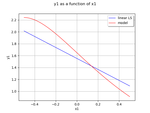
plot 2nd output of our model with x1=0.5

graph = (
    ot.ParametricFunction(responseSurface, [0], [0.5]).getMarginal(1).draw(-0.5, 0.5)
)
graph.setLegends(["linear LS"])
curve = (
    ot.ParametricFunction(model, [0], [0.5])
    .getMarginal(1)
    .draw(-0.5, 0.5)
    .getDrawable(0)
)
curve.setColor("red")
curve.setLegend("model")
graph.add(curve)
graph.setLegendPosition("topright")
view = viewer.View(graph)
plt.show()