Create a linear model

In this example we create a surrogate model using linear model approximation.

The following 2-dimensional function is used in this example .

import openturns as ot
import openturns.viewer as viewer

Generation of the data set

We first generate the data and we add noise to the output observations:

ot.RandomGenerator.SetSeed(0)
distribution = ot.Normal(2)
distribution.setDescription(["x", "y"])
func = ot.SymbolicFunction(["x", "y"], ["2 * x - y + 3 + 0.05 * sin(0.8*x)"])
input_sample = distribution.getSample(30)
epsilon = ot.Normal(0, 0.1).getSample(30)
output_sample = func(input_sample) + epsilon

Linear regression

Let us run the linear model algorithm using the LinearModelAlgorithm class and get the associated results :

algo = ot.LinearModelAlgorithm(input_sample, output_sample)
result = algo.getResult()

Residuals analysis

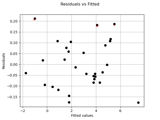
We can now analyse the residuals of the regression on the training data. For clarity purposes, only the first 5 residual values are printed.

residuals = result.getSampleResiduals()
print(residuals[:5])

    [ y0         ]
0 : [  0.186748  ]
1 : [ -0.117266  ]
2 : [ -0.039708  ]
3 : [  0.10813   ]
4 : [ -0.0673202 ]

Alternatively, the standardized or studentized residuals can be used:

stdresiduals = result.getStandardizedResiduals()
print(stdresiduals[:5])

    [ v0        ]
0 : [  1.80775  ]
1 : [ -1.10842  ]
2 : [ -0.402104 ]
3 : [  1.03274  ]
4 : [ -0.633913 ]

Similarly, we can also obtain the underyling distribution characterizing the residuals:

print(result.getNoiseDistribution())

Normal(mu = 0, sigma = 0.110481)

ANOVA table

In order to post-process the linear regression results, the LinearModelAnalysis class can be used:

analysis = ot.LinearModelAnalysis(result)
print(analysis)

Basis( [[x,y]->[1],[x,y]->[x],[x,y]->[y]] )

Coefficients:
           | Estimate    | Std Error   | t value     | Pr(>|t|)    |
--------------------------------------------------------------------
[x,y]->[1] | 2.99847     | 0.0204173   | 146.859     | 9.82341e-41 |
[x,y]->[x] | 2.02079     | 0.0210897   | 95.8186     | 9.76973e-36 |
[x,y]->[y] | -0.994327   | 0.0215911   | -46.0527    | 3.35854e-27 |
--------------------------------------------------------------------

Residual standard error: 0.11048 on 27 degrees of freedom
F-statistic: 5566.3 ,  p-value: 0
---------------------------------
Multiple R-squared   | 0.997581 |
Adjusted R-squared   | 0.997401 |
---------------------------------

---------------------------------
Normality test       | p-value  |
---------------------------------
Anderson-Darling     | 0.456553 |
Cramer-Von Mises     | 0.367709 |
Chi-Squared          | 0.669183 |
Kolmogorov-Smirnov   | 0.578427 |
---------------------------------

The results seem to indicate that the linear hypothesis can be accepted. Indeed, the R-Squared value is nearly 1. Furthermore, the adjusted value, which takes into account the data set size and the number of hyperparameters, is similar to R-Squared.

We can also notice that the Fisher-Snedecor and Student p-values detailed above are lower than 1%. This ensures an acceptable quality of the linear model.

Graphical analyses

Let us compare model and fitted values:

graph = analysis.drawModelVsFitted()
view = viewer.View(graph)

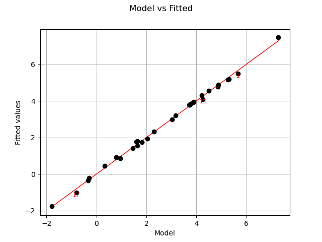
The previous figure seems to indicate that the linearity hypothesis is accurate.

Residuals can be plotted against the fitted values.

graph = analysis.drawResidualsVsFitted()
view = viewer.View(graph)

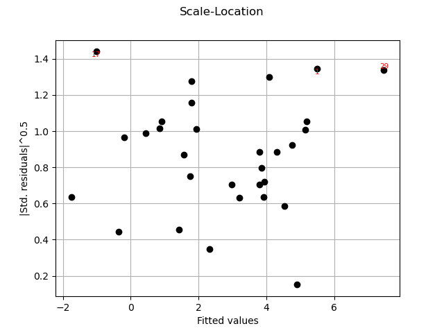
graph = analysis.drawScaleLocation()
view = viewer.View(graph)

graph = analysis.drawQQplot()
view = viewer.View(graph)

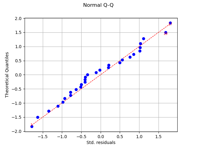
In this case, the two distributions are very close: there is no obvious outlier.

Cook’s distance measures the impact of every invidual data point on the linear regression, and can be plotted as follows:

graph = analysis.drawCookDistance()
view = viewer.View(graph)

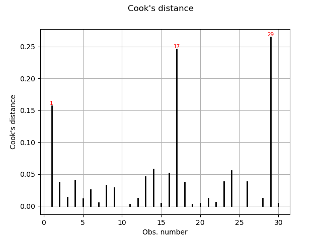
This graph shows us the index of the points with disproportionate influence.

One of the components of the computation of Cook’s distance at a given point is that point’s leverage. High-leverage points are far from their closest neighbors, so the fitted linear regression model must pass close to them.

graph = analysis.drawResidualsVsLeverages()
view = viewer.View(graph)

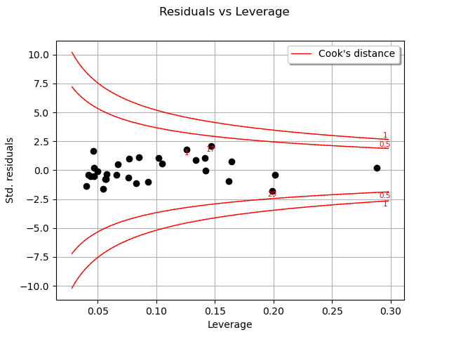
In this case, there seem to be no obvious influential outlier characterized by large leverage and residual values, as is also shown in the figure below:

Similarly, we can also plot Cook’s distances as a function of the sample leverages:

graph = analysis.drawCookVsLeverages()
view = viewer.View(graph)

Finally, we give the intervals for each estimated coefficient (95% confidence interval):

alpha = 0.95
interval = analysis.getCoefficientsConfidenceInterval(alpha)
print("confidence intervals with level=%1.2f : " % (alpha))
print("%s" % (interval))

confidence intervals with level=0.95 :
[2.95657, 3.04036]
[1.97751, 2.06406]
[-1.03863, -0.950026]