Transform a distribution

In this example we are going to use distribution algebra and distribution transformation via functions.

import openturns as ot
import openturns.viewer as viewer
from matplotlib import pylab as plt

ot.Log.Show(ot.Log.NONE)

We define some (classical) distributions :

distribution1 = ot.Uniform(0.0, 1.0)
distribution2 = ot.Uniform(0.0, 2.0)
distribution3 = ot.WeibullMin(1.5, 2.0)

Sum & difference of distributions

It is easy to compute the sum of distributions. For example :

distribution = distribution1 + distribution2
print(distribution)
graph = distribution.drawPDF()
view = viewer.View(graph)

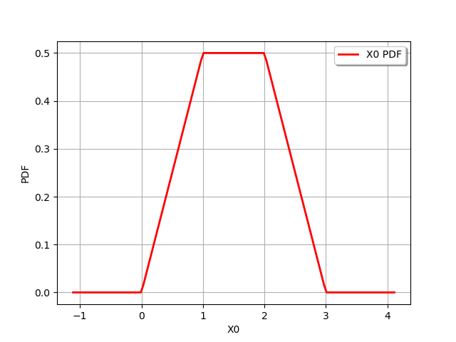
Trapezoidal(a = 0, b = 1, c = 2, d = 3)

We might also use substraction even with scalar values :

distribution = 3.0 - distribution3
print(distribution)
graph = distribution.drawPDF()
view = viewer.View(graph)

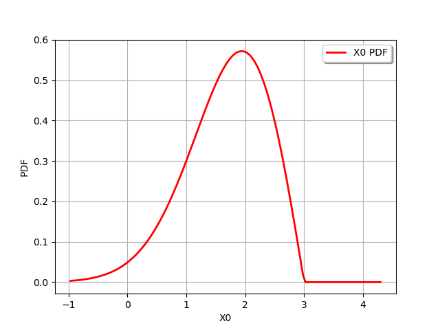
RandomMixture(3 - WeibullMin(beta = 1.5, alpha = 2, gamma = 0))

Product & inverse

We might also compute the product of two (or more) distributions. For example :

distribution = distribution1 * distribution2
print(distribution)
graph = distribution.drawPDF()
view = viewer.View(graph)

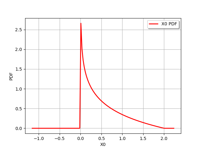
ProductDistribution(Uniform(a = 0, b = 1) * Uniform(a = 0, b = 2))

We could also inverse a distribution :

distribution = 1 / distribution1
print(distribution)
graph = distribution.drawPDF()
view = viewer.View(graph)

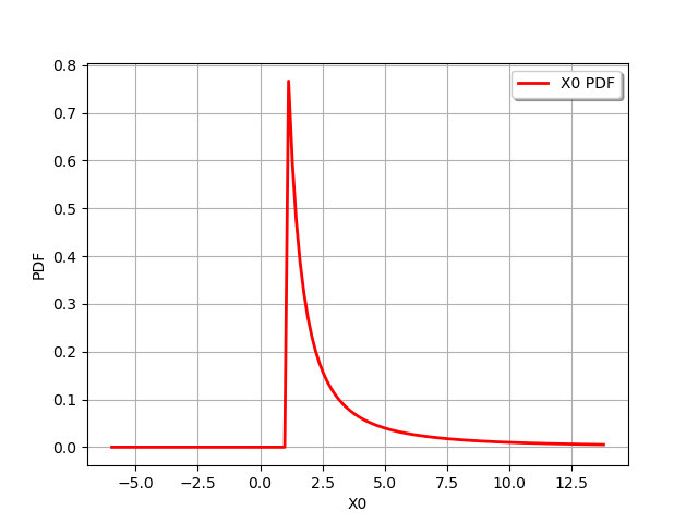
CompositeDistribution=f(Uniform(a = 0, b = 1)) with f=[x]->[1.0 / x]

Or compute a ratio distribution :

ratio = distribution2 / distribution1
print(ratio)
graph = ratio.drawPDF()
view = viewer.View(graph)

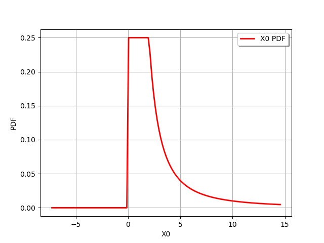
ProductDistribution(Uniform(a = 0, b = 2) * CompositeDistribution=f(Uniform(a = 0, b = 1)) with f=[x]->[1.0 / x])

Transformation using functions

The library provides methods to get the full distributions of f(x) where f can be equal to :

• sin,

• asin,

• cos,

• acos,

• tan,

• atan,

• sinh,

• asinh,

• cosh,

• acosh,

• tanh,

• atanh,

• sqr (for square),

• inverse,

• sqrt,

• exp,

• log/ln,

• abs,

• cbrt.

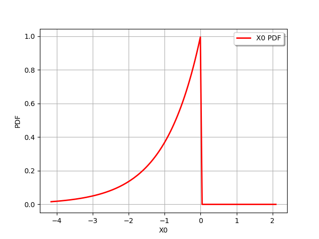
For example for the usual log transformation :

graph = distribution1.log().drawPDF()
view = viewer.View(graph)

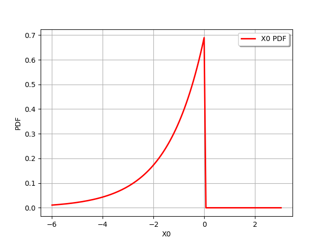
And for the log2 function :

f = ot.SymbolicFunction(["x"], ["log2(x)"])
f.setDescription(["X", "ln(X)"])
graph = ot.CompositeDistribution(f, distribution1).drawPDF()
view = viewer.View(graph)

If one wants a specific method, user might rely on the CompositeDistribution class.

# Create a composite distribution
# -------------------------------
#
# In this paragraph we create a distribution defined as the push-forward distribution of a scalar distribution by a transformation.
#
# If we note :math:`\mathcal{L}_0` a scalar distribution, :math:`f: \mathbb{R} \rightarrow \mathbb{R}` a mapping, then it is possible to create the push-forward distribution :math:`\mathcal{L}` defined by
#
# .. math::
#    \mathcal{L} = f(\mathcal{L}_0)
#

We create a 1D normal distribution :

antecedent = ot.Normal()

and a 1D transform :

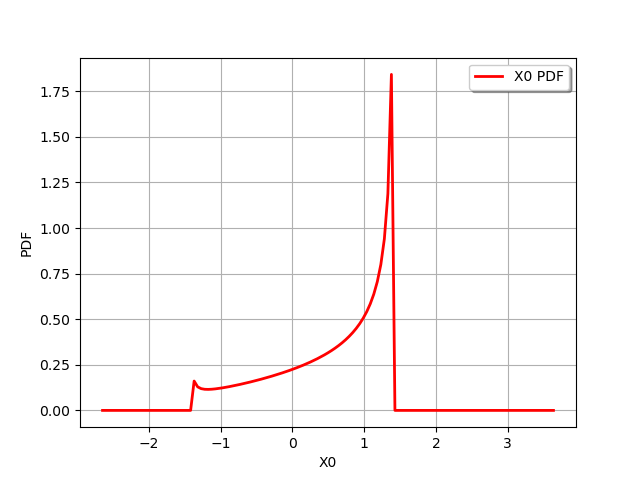
f = ot.SymbolicFunction(["x"], ["sin(x)+cos(x)"])

We then create the composite distribution :

distribution = ot.CompositeDistribution(f, antecedent)
graph = distribution.drawPDF()
view = viewer.View(graph)

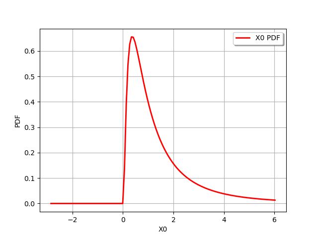
We can also build a distribution with the simplified construction :

distribution = antecedent.exp()
graph = distribution.drawPDF()
view = viewer.View(graph)

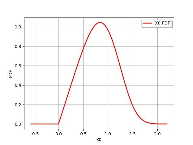
and by using chained operators :

distribution = antecedent.abs().sqrt()
graph = distribution.drawPDF()
view = viewer.View(graph)

Display all figures

plt.show()