Note

Go to the end to download the full example code

Linear Regression with interval-censored observations¶

1. Model formulation¶

We consider the following linear model:

$\vect{Y} = \mat{X} \vect{\theta} + \vect{\varepsilon},$

where the observation vector $\vect{Y} \in \mathbb R^{n}$ is modeled as the sum of:

a linear part, with an $n \times p$ design matrix $\mat{X}$ and unknown regression coefficients $\vect{\theta} \in\mathbb R^p$ ,
a Gaussian error term $\vect{\varepsilon} \sim \mathcal N_n(\vect{0}, \tau^{-1} \mat{I}_n+\mat{Q}^{-1})$ ,

where $\mat{Q}$ represents a known precision (inverse variance) matrix for measurement errors, and $\tau$ an unknown precision parameter quantifying the variability of the observed phenomenon.

1.1. Likelihood of the linear regression model¶

The above linear regression model can thus be written:

$\vect{Y} | \vect{\theta}, \tau {\sim} \mathcal N_{n}(\mat{X} \vect{\theta} ; \tau^{-1} \mat{I}_n +\mat{Q}^{-1}),$

We then have the following likelihood:

$\mathcal L(\vect{Y}|\vect{\theta}, \tau) = (2\pi)^{-\frac{n}{2}} {\rm det}(\tau^{-1} \mat{I}_n+\mat{Q}^{-1})^{-\frac{1}{2}} e^{-\frac{1}{2} ||\vect{Y} - \mat{X} \vect{\theta} ||_{\tau^{-1} \mat{I}_n +\mat{Q}^{-1}}^2 }$

where $||\vect{X}-\vect{Y}||_{\mat{V}}^2$ is the Mahalanobis distance between $\vect{X}$ and $\vect{Y}$ with covariance matrice $\mat{V}$ :

$||\vect{X}-\vect{Y}||_{\mat{V}}^2 = (\vect{X}-\vect{Y})^\top\ \mat{V}^{-1}\ (\vect{X}-\vect{Y}).$

1.2. Interval Censorship¶

We now assume that, instead of observing directly the $Y_i, i=1,\ldots,n$ as described above, we only have access to discretized values $Y_i^{obs} \in \delta \times \mathbb N$ , where $\delta > 0$ is a grid length and $Y_i^{obs} = \delta \times k$ means that $Y_i \in \delta \times \left[ k - \frac{1}{2}; k + \frac{1}{2} \right[$ .

1.3. Remarks¶

The presence of a composite matrix $\tau^{-1} \mat{I}_n+\mat{Q}^{-1}$ makes estimation more complex than with a spherical one $\tau^{-1}\mat{I}_n,$ since we would then have explicit (closed-form) maximum likelihood estimators, and also conjugate priors leading to explicit full joint posterior distributions.
Another difficulty is the presence of censored data, since the likelihood is no more available in closed-form. As we will see, this can be overcome thanks to Bayesian inference.
Heteroscedastic linear modeling under interval censorship as formulated above was originally motivated by an industrial case-study in seismology, wherein the $Y_i$ correspond to the observed intensity of an earthquake in a distant site, and explanatory variables $\vect{X}_{i}$ are derived from the epicentral distance to the earthquake’s source as well as its characteristics (magnitude, depth). But it can also arise in many different contexts, as soon as observations are available with known statistical precisions (hence the heteroscedasticity) and limited numerical accuracy (hence the censorship).

1.4 Simulate the dataset¶

import openturns as ot
from openturns.viewer import View
import numpy as np

ot.Log.Show(ot.Log.NONE)
ot.RandomGenerator.SetSeed(1)

n = 10
delta = 0.5

Build the design matrix $\mat{X}$

X = ot.Sample([[1.0]] * n)
X.stack(ot.Normal(0.0, 10.0).getSample(n))

Make the precision matrix $\mat{Q}$ a diagonal matrix and sample its diagonal coefficients from an Exponential distribution.

Q = np.ones((n, 1)) + ot.Exponential().getSample(n)

Choose values for the parameters $\vect{\theta}$ and $\tau$ .

theta_true = np.array([[0.0], [1.0]])
p = len(theta_true)
tau_true = 0.1

First sample uncensored, and then censored observation data.

mean_true = np.dot(X, theta_true).ravel()
std_true = np.sqrt(1.0 / tau_true + 1.0 / Q).ravel()

Y_sim = mean_true + [x[0] for x in ot.Normal().getSample(n)] * std_true
Yobs_sim = np.round(Y_sim / delta) * delta

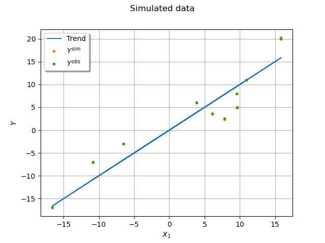
Plot the simulated dataset.

graph = ot.Graph("Simulated data", "$X_1$", "$Y$", True, "topleft", 16)
cloud_obs = ot.Cloud(X[:, 1].asPoint(), Yobs_sim)
cloud_obs.setPointStyle("bullet")
cloud_sim = ot.Cloud(X[:, 1].asPoint(), Y_sim)
cloud_sim.setPointStyle("bullet")
curve = ot.Curve(X[:, 1].asPoint(), mean_true)
curve.setLineWidth(1.5)
graph.add(curve)
graph.add(cloud_sim)
graph.add(cloud_obs)
graph.setLegends(["Trend", "$Y^{sim}$", "$Y^{obs}$"])
graph.setColors(ot.Drawable.BuildDefaultPalette(3))
_ = View(graph)

2. Bayesian Inference¶

2.1. Choice of a prior law¶

We use the standard Normal-Gamma prior for $\vect{\theta}$ and $\tau$ :

$\vect{\theta} | \tau \sim \mathcal N_{p}(\vect{\mu}_0; \tau^{-1}\mat{\Sigma}_0) \\ \tau \sim \mathcal G(a_0, b_0),$

where all parameters are assumed a priori independent if not stated otherwise.

Furthermore, a default choice for the hyperparameters consists in having all prior variances go to infinity, equivalent to the degenerate case:

$\vect{\mu}_0, \mat{\Sigma}_0^{-1}, a_0, b_0 \equiv 0$

But the resulting prior is improper. Hence, posterior propriety needs to be proven first.

A simpler solution is to ensure prior (hence posterior) propriety by imposing bounds $\vect{\theta}_{\min}, \vect{\theta}_{\max}, \tau_{\min}, \tau_{\max}$ on all parameters following:

$\vect{\theta} | \tau \sim \mathcal N_{p}(\vect{\mu}_0; \tau^{-1}\mat{\Sigma}_0) {\bf 1}_{\{\vect{\theta}_{\min} \leq \vect{\theta} \leq \vect{\theta}_{\max}\}} ;\\ \tau \sim \mathcal G(a_0, b_0){\bf 1}_{\{\tau_{\min} \leq \tau \leq \tau_{\max}\}},$

where inequalites are taken componentwise. When all hyperparameters go to $0$ as described above, the prior converges to a product of uniform distributions.

We will use this product of univariate uniforms as a prior in the following. As discussed above, there is no simple way to obtain the posterior distribution, justifying the use of Monte-Carlo Markov chain techniques, as described hereafter.

lower = (Yobs_sim.ravel() - delta).tolist()
upper = (Yobs_sim.ravel() + delta).tolist()

# Global support of the joint distribution: theta, tau, outputs
support = ot.Interval([-2.0] * p + [1e-4] + lower, [2.0] * p + [1e1] + upper)

prior = ot.ComposedDistribution(
    [ot.Uniform(-2.0, 2.0), ot.Uniform(-2.0, 2.0), ot.Uniform(1e-4, 1e1)]
)

# Initialize to true value
initial_state = theta_true[:, 0].tolist() + [tau_true] + Y_sim.ravel().tolist()
initial_state = ot.Point(initial_state)

2.2. Posterior sampling¶

The solution we advocate consists in sampling from the joint posterior distribution of all uncertain parameters, including the vector of continuous intensities $\vect{Y},$ seen here as a latent variable. Indeed, adding $\vect{Y}$ to the vector of sampled variables yields a posterior density which is available in closed form, up to an unknown multiplicative factor

$\begin{array}{ll} \pi(\vect{Y},\vect{\theta},\tau|\vect{Y}^{obs}) & \propto \pi(\vect{\theta},\tau)\times\mathcal L(\vect{Y}|\vect{\theta},\tau)\mathcal L(\vect{Y}^{obs}|\vect{Y})\\ & \propto {\bf 1}_{\{\vect{\theta}_{\min} \leq \vect{\theta} \leq \vect{\theta}_{\max}\}}\times {\bf 1}_{\{\tau_{\min} \leq \tau \leq \tau_{\max}\}}\times \mathcal N_n (\vect{Y}|\mat{X} \vect{\theta};\tau^{-1} \mat{I}_n + \mat{Q}^{-1}) \times {\bf 1}_{\left[\vect{Y}^{obs}-\frac{\delta}{2}; \vect{Y}^{obs}+\frac{\delta}{2}\right[}(\vect{Y}). \end{array}$

This allows one to perform the following Metropolis within Gibbs sampling scheme, wherein the pre-defined blocks of variables $(\vect{Y},\vect{\theta},\tau)$ are updated in turn, according to their conditional posterior density, or to a Markov kernel targeting it, as described in the following.

2.2.1. Updating $\vect{Y}$ ¶

$\pi(\vect{Y}|\vect{\theta},\tau,\vect{Y}^{obs})\propto\prod_{i=1}^{n}\mathcal N(Y_{i}|\vect{X}_{i} \vect{\theta}, \tau^{-1}+q_{i}^{-1}) {\bf 1}_{\left[Y_{i}^{obs}-\frac{\delta}{2}; Y_{i}^{obs}+\frac{\delta}{2}\right[}(Y_{i})$

hence the latent variables $Y_i$ are updated by simply simulating independent univariate truncated normals.

Step 1 : Create associated RandomVector

marginals_trunc = [
    ot.TruncatedNormal(Yobs_sim[i], 1.0, lower[i], upper[i]) for i in range(len(X))
]

trunc_cond_Y = ot.ComposedDistribution(marginals_trunc)
RV_Y = ot.RandomVector(trunc_cond_Y)

Step 2 : Link function, giving the parameters of the univariate truncated normals in function of the chain’s current state

gen_params = np.array(trunc_cond_Y.getParameter())


def py_link_function_y(x):
    """
    link function for Y conditional density

    Input
        x: vector with length (p + 1 + n), containing the current state of (theta, tau, Y)

    Output
        params: vector with length 4*n, corresponding to mean, std, a and b, for each component of Y

    Notes
        a and b represent the upper and lower bounds for the truncated normals
    """
    theta = [x[i] for i in range(p)]
    tau = x[p]
    # compute conditional mean and standard deviates
    mean = np.dot(X, theta)
    std = np.sqrt(1.0 / tau + 1.0 / Q)
    # inject values in blueprint
    params = gen_params.copy()
    params[::4] = mean
    params[1::4] = std.ravel()
    return params

2.2.2. Updating $\vect{\theta}$ ¶

$\pi(\vect{\theta}|\vect{Y}, \tau, \vect{Y}^{obs})=\pi(\vect{\theta}|\vect{Y},\tau).$ Due to the partial conjugacy of the conditional prior $\pi(\vect{\theta}|\tau),$ this is explicit, and given by the following box-constrained multivariate normal:

$\vect{\theta}|\vect{Y},\tau \sim \mathcal N_4( \vect{\mu}_n ; \mat{\Sigma}_n ){\bf 1}_{\{\vect{\theta}_{\min} \leq \vect{\theta} \leq \vect{\theta}_{\max}\}},$

with

$\vect{\mu}_n = \vect{\mu}_0 + \mat{\Sigma}_0X^\top(\mat{X} \mat{\Sigma}_0 \mat{X}^\top + \mat{I}_n + \tau \mat{Q}^{-1})^{-1}(\vect{Y} - \mat{X} \vect{\mu}_0) \\ \mat{\Sigma}_n = \tau^{-1}\mat{\Sigma}_0 - \tau^{-1}\mat{\Sigma}_0 \mat{X}^\top (\mat{X} \mat{\Sigma}_0 \mat{X}^\top + \mat{I}_n + \tau \mat{Q}^{-1})^{-1} \mat{X} \mat{\Sigma}_0,$

or equivalently, thanks to the matrix Woodsbury identity:

$\vect{\mu}_n = (\mat{\Sigma}_0^{-1} + \mat{X}^\top (\mat{I}_n + \tau \mat{Q}^{-1})^{-1} \mat{X})^{-1}(\mat{\Sigma}_0^{-1} \vect{\mu}_0 + \mat{X}^\top (\mat{I}_n + \tau \mat{Q}^{-1})^{-1} \vect{Y})\\ \mat{\Sigma}_n = \tau^{-1}(\mat{\Sigma}_0^{-1} + \mat{X}^\top (\mat{I}_n + \tau \mat{Q}^{-1})^{-1} \mat{X})^{-1}.$

By having all hyperparameters go to $0,$ we obtain the following simplified form:

$\vect{\mu}_n = (\mat{X}^\top (\mat{I}_n + \tau \mat{Q}^{-1})^{-1} \mat{X})^{-1}(\mat{X}^\top (\mat{I}_n + \tau \mat{Q}^{-1})^{-1} \vect{Y})\\ \mat{\Sigma}_n = \tau^{-1}(\mat{X}^\top (\mat{I}_n + \tau \mat{Q}^{-1})^{-1} \mat{X})^{-1}.$

Explicit simulation from a box-constrained multivariate normal can be done with a simple rejection sampling scheme:

Step 1 : Create associated RandomVector

class BoxConstrainedNormal(ot.PythonRandomVector):
    """
    Multivariate normal distribution
    under box constraints
    """

    def __init__(
        self, d=2, mu=np.zeros(2), Sigma=np.eye(2), r=np.zeros(2), s=np.ones(2)
    ):
        for x in mu, Sigma, r, s:
            if len(x) != d:
                print("expectation or bound does not have size %s" % d)
                raise ValueError
        if Sigma.shape != (d, d):
            print("covariance matrix not have dimensions (%s,%s)" % (d, d))
            raise ValueError
        super(BoxConstrainedNormal, self).__init__(d)
        self.mu = mu
        self.Sigma = Sigma
        self.r = r
        self.s = s
        self.interval = ot.Interval(r, s)

    def setParameter(self, parameter):
        d = self.getDimension()
        self.mu = np.array(parameter[:d])
        self.Sigma = np.array(parameter[d: d + d * d]).reshape(d, d)
        self.r = np.array(parameter[-2 * d: -d])
        self.s = np.array(parameter[-d:])
        self.interval = ot.Interval(self.r, self.s)

    def getParameter(self):
        return np.concatenate(
            [self.mu.ravel(), self.Sigma.ravel(), self.r.ravel(), self.s.ravel()]
        )

    def getRealization(self):
        accept = False
        proposaldist = ot.Normal(self.mu, ot.CovarianceMatrix(self.Sigma))
        while not accept:
            proposal = proposaldist.getRealization()
            accept = self.interval.contains(proposal)
        return proposal


RV_theta = ot.RandomVector(BoxConstrainedNormal())

Step 2 : Link function, giving the parameters of the box-constrained normal in function of $\tau$ and $\vect{Y}$ values

def py_link_function_theta(x):
    tau = x[p]
    Y = [x[i] for i in range(p + 1, len(x))]
    # conditional mean and variance
    # for diagonal Q
    Itilde_inv = 1.0 / (1.0 + tau / Q)
    Xtilde = Itilde_inv * X
    Sigma_n = np.linalg.inv(np.dot(Xtilde.T, X)) / tau
    mu_n = np.dot(Xtilde.T, Y)
    mu_n = tau * np.dot(Sigma_n, mu_n)
    # extract parameters in correct order (coherent with getParameter() method of RV_theta)
    return np.concatenate(
        [
            mu_n.ravel(),
            Sigma_n.ravel(),
            support.getLowerBound()[:p],
            support.getUpperBound()[:p],
        ]
    )

2.2.3. Updating $\tau$ ¶

$\pi(\tau|\vect{Y},\vect{\theta})$ is proportional to:

$\pi(\tau|\vect{Y},\vect{\theta}) \propto {\bf 1}_{\{\tau_{\min} \leq \tau \leq \tau_{\max}\}}\times \mathcal N_n(\vect{Y}|\mat{X} \vect{\theta};\tau^{-1} \mat{I}_n + \mat{Q}^{-1}).$

Hence, $\tau$ can be updated using the Random-walk Metropolis-Hastings algorithm.

Step 1 : compute tau’s conditional posterior density, up to a multiplicative factor

def marginals_Y(theta, tau):
    mu = np.dot(X, theta).ravel()
    sigma = np.sqrt(1.0 / tau + 1.0 / Q).ravel()
    return [ot.Normal(mu[i], sigma[i]) for i in range(len(X))]


def py_log_density(x):
    theta = [x[i] for i in range(p)]
    tau = x[p]
    Y = [x[p + 1 + i] for i in range(len(X))]
    ld = ot.ComposedDistribution(marginals_Y(theta, tau)).computeLogPDF(Y)
    return [ld]

Step 2 : define the proposal distribution

proposal_tau = ot.Normal(0.0, 1e-1)

2.3. Initialization¶

To avoid all numerical problems, it is better to provide the algorithm with a starting point not too far from the posterior mode. To this end, we propose to set $\vect{Y}=\vect{Y}^{obs}$ for simplicity, then solve the following optimization problem

$\widehat\theta,\widehat\tau = \arg\max_{\vect{\theta},\tau} \pi(\vect{\theta},\tau|\vect{Y}^{obs},\vect{Y}=\vect{Y}^{obs}) = \arg\max_{\theta\in[\vect{\theta}_{\min};\vect{\theta}_{\max}] \tau\in[\tau_{\min};\tau_{\max}]} \mathcal N(\vect{Y}^{obs}|\vect{\theta} \mat{X}; \tau^{-1} \mat{I}_n + \mat{Q}^{-1}).$

Note that the unconstrained optimization over $\vect{\theta}$ for fixed $\tau$ is explicit, since:

$\arg\max_{\vect{\theta}} \pi(\vect{\theta},\tau|\vect{Y}^{obs},\vect{Y}=\vect{Y}^{obs}) =\arg\max_{\vect{\theta}} \pi(\vect{\theta}|\vect{Y}^{obs},\vect{Y}=\vect{Y}^{obs},\tau).$

But we have shown that the conditional posterior density of $\vect{\theta}$ is Gaussian. Hence the unconstrained conditional posterior mode (and mean) is given by:

$\arg\max_{\vect{\theta}} \pi(\vect{\theta}|\vect{Y}^{obs},\vect{Y}=\vect{Y}^{obs},\tau) = (\mat{X}^\top (\mat{I}_n + \tau \mat{Q}^{-1})^{-1} \mat{X})^{-1}(\mat{X}^\top (\mat{I}_n + \tau \mat{Q}^{-1})^{-1} \vect{Y}):= \vect{\mu}_n(\tau).$

If this point does not respect the constraints, then we simply project each component unto the constrained space.

Hence the following 1D problem remains to be solved:

$\widehat\tau = \arg\max_{\tau\in[\tau_{\min};\tau_{\max}]} \mathcal N(\vect{Y}^{obs}|\vect{\mu}_n(\tau) \mat{X}; \tau^{-1} \mat{I}_n + \mat{Q}^{-1}).$

The optimal value of $\vect{\theta}$ is then given by: $\widehat{\vect{\theta}} = \vect{\mu}_n(\widehat\tau).$

def mu_n(tau):
    x = ot.Point(initial_state)
    x[p] = tau
    # trick: posterior conditional mean is computed by the link function
    return py_link_function_theta(x)[:p]


# optimization criterion
def log_cond_tau_post(tau):
    x = ot.Point(initial_state)
    x[p] = tau
    # replace theta by its conditional posterior mean
    x[:p] = py_link_function_theta(x)[:p]
    # compute log conditional posterior of tau
    ll = py_log_density(x)[0]
    return ll

1D optimization

def func(X):
    return [-log_cond_tau_post(X[0])]


problem = ot.OptimizationProblem(ot.PythonFunction(1, 1, func))
problem.setBounds(ot.Interval([1e-4], [1e4]))
solver = ot.TNC(problem)
solver.setStartingPoint([1.0])
solver.run()
tauhat = solver.getResult().getOptimalPoint()[0]
print("tauhat =", tauhat)

# inject result in initialState vector
x = ot.Point(initial_state)
x[:p] = mu_n(tauhat)
x[p] = tauhat

tauhat = 0.10077295009614318

Final step : create a MetropolisHastings object for each block

initialState = x

mi_Y = [i for i in range(p + 1, p + 1 + n)]
link_function_y = ot.PythonFunction(len(x), 4 * n, py_link_function_y)
rvmh_Y = ot.RandomVectorMetropolisHastings(RV_Y, initialState, mi_Y, link_function_y)

mi_theta = [i for i in range(p)]
link_function_theta = ot.PythonFunction(len(x), p + (p + 2) * p, py_link_function_theta)
rvmh_theta = ot.RandomVectorMetropolisHastings(
    RV_theta, initialState, mi_theta, link_function_theta
)

log_pdf_tau = ot.PythonFunction(len(x), 1, py_log_density)
rwmh_tau = ot.RandomWalkMetropolisHastings(
    log_pdf_tau, support, initialState, proposal_tau, [p]
)

# Now, assemble the blocks to create a Gibbs algorithm:
gibbs = ot.Gibbs([rvmh_Y, rvmh_theta, rwmh_tau])

Launch Algorithm

sampleSize = 1000

# Joint posterior density sample
sample = gibbs.getSample(sampleSize)

# compute acceptance rate
tau_post = np.array(sample[:, p]).ravel()
acc_rate = (tau_post[1:] != tau_post[:-1]).mean()
print("Acceptance rate: %s" % acc_rate)

Acceptance rate: 0.32732732732732733

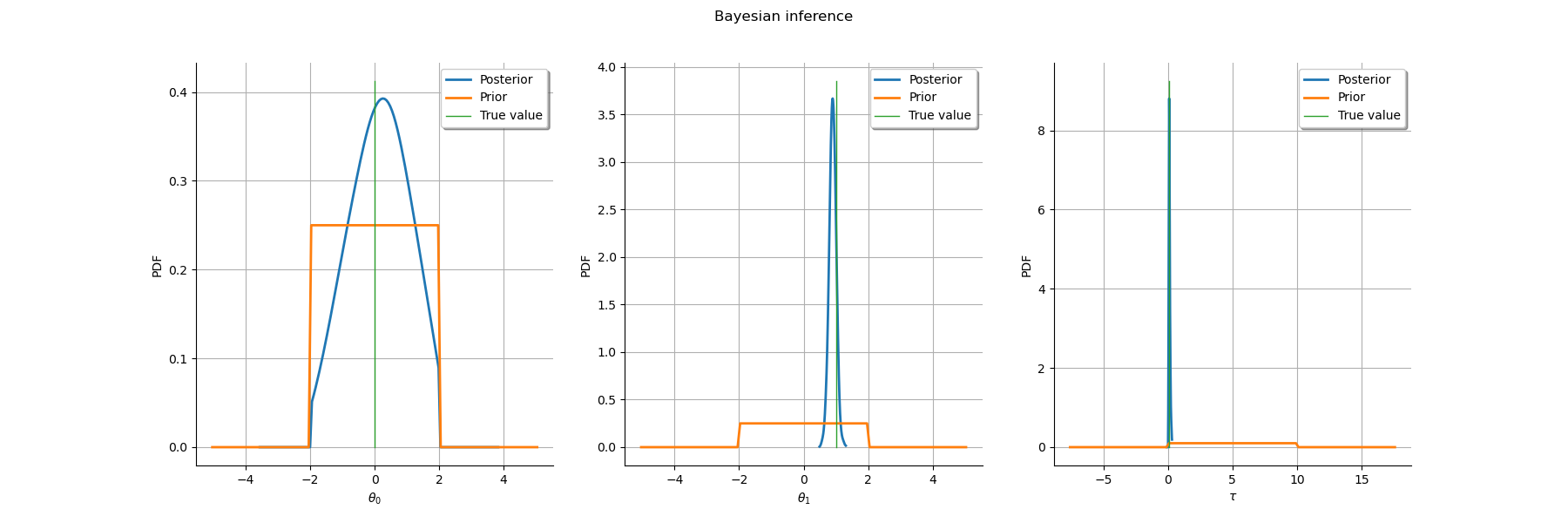
Plot posterior distribution marginals

# extract interest parameters
post_sample = sample.getMarginal([i for i in range(p + 1)])
post_sample.setDescription(["$\\theta_0$", "$\\theta_1$", "$\\tau$"])

posterior = ot.KernelSmoothing().build(post_sample)
posterior = ot.TruncatedDistribution(posterior, prior.getRange())

grid = ot.GridLayout(1, 3)
grid.setTitle("Bayesian inference")
xlabs = [r"$\theta_0$", r"$\theta_1$", r"$\tau$"]
p_true = [theta_true[0][0], theta_true[1][0], tau_true]
for parameter_index in range(3):
    graph = posterior.getMarginal(parameter_index).drawPDF()
    bbox = graph.getBoundingBox()
    bound = bbox.getUpperBound()[1]
    prior_pdf = prior.getMarginal(parameter_index).drawPDF()
    graph.add(prior_pdf)
    curve_true = ot.Curve([p_true[parameter_index]] * 2, [0.0, bound])
    graph.add(curve_true)
    graph.setColors(ot.Drawable.BuildDefaultPalette(3))
    graph.setLegends(["Posterior", "Prior", "True value"])
    graph.setXTitle(xlabs[parameter_index])
    grid.setGraph(0, parameter_index, graph)
_ = View(grid)

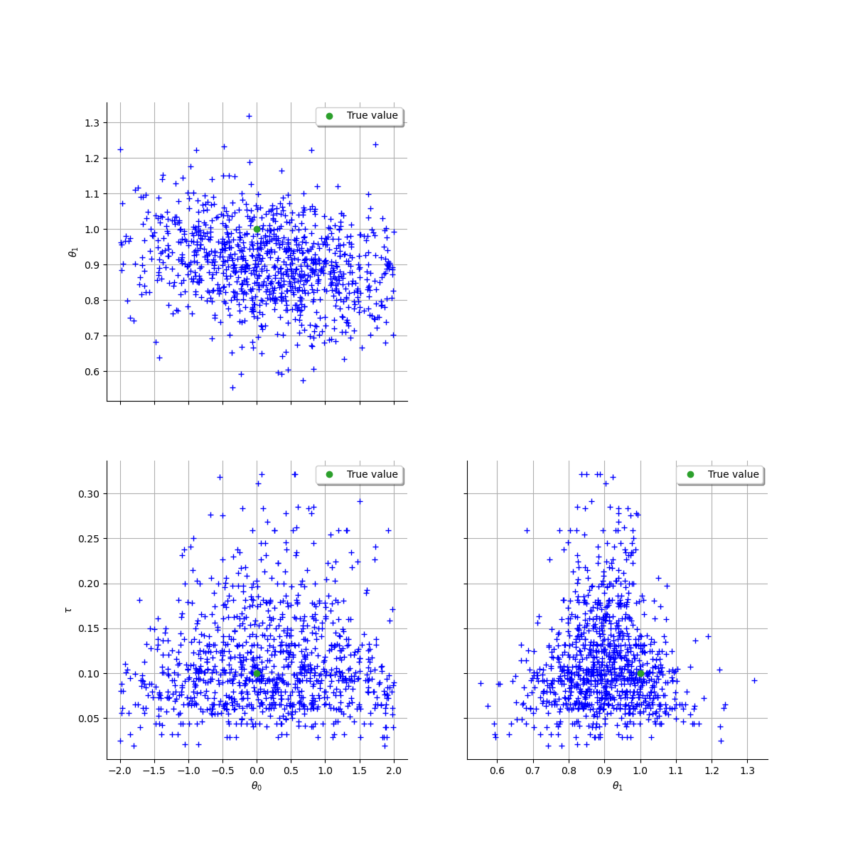
Draw pairplots of the posterior sample.

# sphinx_gallery_thumbnail_number = 3
grid = ot.VisualTest.DrawPairs(post_sample)

graph = grid.getGraph(0, 0)
pt = ot.Cloud(theta_true.T, "#2ca02c", "circle", "True value")
graph.add(pt)
grid.setGraph(0, 0, graph)

graph = grid.getGraph(1, 0)
pt = ot.Cloud([[theta_true[0, 0], tau_true]], "#2ca02c", "circle", "True value")
graph.add(pt)
grid.setGraph(1, 0, graph)

graph = grid.getGraph(1, 1)
pt = ot.Cloud([[theta_true[1, 0], tau_true]], "#2ca02c", "circle", "True value")
graph.add(pt)
grid.setGraph(1, 1, graph)

_ = View(grid)


View.ShowAll()

OpenTURNS

An Open source initiative for the Treatment of Uncertainties, Risks'N Statistics

Table of Contents

Previous topic

Next topic

This Page

Linear Regression with interval-censored observations¶

1. Model formulation¶

1.1. Likelihood of the linear regression model¶

1.2. Interval Censorship¶

1.3. Remarks¶

1.4 Simulate the dataset¶

2. Bayesian Inference¶

2.1. Choice of a prior law¶

2.2. Posterior sampling¶

2.2.1. Updating $\vect{Y}$ ¶

2.2.2. Updating $\vect{\theta}$ ¶

2.2.3. Updating $\tau$ ¶

2.3. Initialization¶

OpenTURNS

An Open source initiative for the Treatment of Uncertainties, Risks'N Statistics

Linear Regression with interval-censored observations¶

1. Model formulation¶

1.1. Likelihood of the linear regression model¶

1.2. Interval Censorship¶

1.3. Remarks¶

1.4 Simulate the dataset¶

2. Bayesian Inference¶

2.1. Choice of a prior law¶

2.2. Posterior sampling¶

2.2.1. Updating ¶

2.2.2. Updating ¶

2.2.3. Updating ¶

2.3. Initialization¶

2.2.1. Updating $\vect{Y}$ ¶

2.2.2. Updating $\vect{\theta}$ ¶

2.2.3. Updating $\tau$ ¶