Note
Go to the end to download the full example code
Estimate Wilks and empirical quantile
In this example we want to evaluate a particular quantile, with the empirical estimator or the Wilks one, from a sample of a random variable.
Let us suppose we want to estimate the quantile of order
of the variable
:
, from the sample
of size
, with a confidence level equal to
.
We note the sample where the values are sorted in ascending order.
The empirical estimator, noted
, and its confidence interval, is defined by the expressions:
The Wilks estimator, noted , and its confidence interval, is defined by the expressions:
Once the order has been chosen, the Wilks number
is evaluated,
thanks to the static method
of the Wilks object.
In the example, we want to evaluate a quantile ,
with a confidence level of
thanks to the
).
Be careful: means that the Wilks estimator is the maximum of the sample:
it corresponds to the first maximum of the sample.
import openturns as ot
import math as m
import openturns.viewer as viewer

ot.Log.Show(ot.Log.NONE)
model = ot.SymbolicFunction(["x1", "x2"], ["x1^2+x2"])
R = ot.CorrelationMatrix(2)
R[0, 1] = -0.6
inputDist = ot.Normal([0.0, 0.0], R)
inputDist.setDescription(["X1", "X2"])
inputVector = ot.RandomVector(inputDist)

# Create the output random vector Y=model(X)
output = ot.CompositeRandomVector(model, inputVector)
Quantile level
alpha = 0.95

# Confidence level of the estimation
beta = 0.90
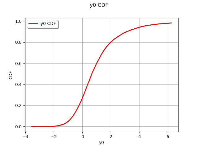
Get a sample of the variable
N = 10 ** 4
sample = output.getSample(N)
graph = ot.UserDefined(sample).drawCDF()
view = viewer.View(graph)

Empirical Quantile Estimator
empiricalQuantile = sample.computeQuantile(alpha)

# Get the indices of the confidence interval bounds
aAlpha = ot.Normal(1).computeQuantile((1.0 + beta) / 2.0)[0]
min_i = int(N * alpha - aAlpha * m.sqrt(N * alpha * (1.0 - alpha)))
max_i = int(N * alpha + aAlpha * m.sqrt(N * alpha * (1.0 - alpha)))
# print(min_i, max_i)

# Get the sorted sample
sortedSample = sample.sort()

# Get the Confidence interval of the Empirical Quantile Estimator [infQuantile, supQuantile]
infQuantile = sortedSample[min_i - 1]
supQuantile = sortedSample[max_i - 1]
print(infQuantile, empiricalQuantile, supQuantile)
[4.13903] [4.28037] [4.35925]
Wilks number
i = N - (min_i + max_i) // 2  # compute wilks with the same sample size
wilksNumber = ot.Wilks.ComputeSampleSize(alpha, beta, i)
print("wilksNumber =", wilksNumber)
wilksNumber = 10604
Wilks Quantile Estimator
algo = ot.Wilks(output)
wilksQuantile = algo.computeQuantileBound(alpha, beta, i)
print("wilks Quantile 0.95 =", wilksQuantile)
wilks Quantile 0.95 = [4.37503]
 OpenTURNS