Compute SRC indices confidence intervals

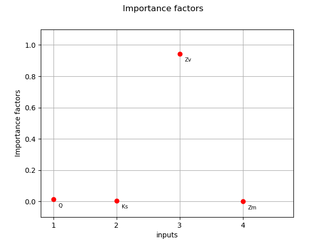
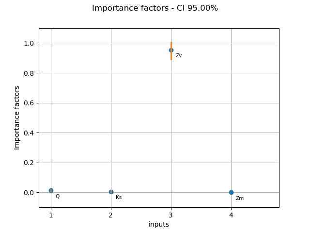
This example shows how to compute SRC indices confidence bounds with bootstrap. First, we compute SRC indices and draw them. Then we compute bootstrap confidence bounds using the BootstrapExperiment class and draw them.

import openturns as ot
import openturns.viewer as otv
from openturns.usecases import flood_model

Load the flood model.

flood = flood_model.FloodModel()
distribution = flood.distribution
g = flood.model
dim = distribution.getDimension()

We produce a pair of input and output sample.

ot.RandomGenerator.SetSeed(0)
N = 100
X = distribution.getSample(N)
Y = g(X)

Compute SRC indices from the generated design.

importance_factors = ot.CorrelationAnalysis(X, Y).computeSquaredSRC()
print(importance_factors)

[0.0129289,0.00545588,0.943028,0.000193272]

Plot the SRC indices.

input_names = g.getInputDescription()
graph = ot.SobolIndicesAlgorithm.DrawCorrelationCoefficients(
    importance_factors, input_names, "Importance factors"
)
graph.setYTitle("Importance factors")
_ = otv.View(graph)

We now compute bootstrap confidence intervals for the importance factors. This is done with the BootstrapExperiment class.

Create SRC bootstrap sample

bootstrap_size = 100
src_boot = ot.Sample(bootstrap_size, dim)
for i in range(bootstrap_size):
    selection = ot.BootstrapExperiment.GenerateSelection(N, N)
    X_boot = X[selection]
    Y_boot = Y[selection]
    src_boot[i, :] = ot.CorrelationAnalysis(X_boot, Y_boot).computeSquaredSRC()

Compute bootstrap quantiles

alpha = 0.05
src_lb = src_boot.computeQuantilePerComponent(alpha / 2.0)
src_ub = src_boot.computeQuantilePerComponent(1.0 - alpha / 2.0)
src_interval = ot.Interval(src_lb, src_ub)
print(src_interval)

[0.0090078, 0.0180504]
[0.00292053, 0.012593]
[0.891574, 1.00615]
[4.51853e-05, 0.000459976]

def draw_importance_factors_with_bounds(
    importance_factors, input_names, alpha, importance_bounds
):
    """
    Plot importance factors indices with confidence bounds of level 1 - alpha.

    Parameters
    ----------
    importance_factors : Point(dimension)
        The importance factors.
    input_names : list(str)
        The names of the input variables.
    alpha : float, in [0, 1]
        The complementary confidence level.
    importance_bounds : Interval(dimension)
        The lower and upper bounds of the importance factors

    Returns
    -------
    graph : Graph
        The importance factors indices with lower and upper 1-alpha confidence intervals.
    """
    dim = importance_factors.getDimension()
    lb = importance_bounds.getLowerBound()
    ub = importance_bounds.getUpperBound()
    palette = ot.Drawable.BuildDefaultPalette(2)
    graph = ot.SobolIndicesAlgorithm.DrawCorrelationCoefficients(
        importance_factors, input_names, "Importance factors"
    )
    graph.setColors([palette[0], "black"])
    graph.setYTitle("Importance factors")

    # Add confidence bounds
    for i in range(dim):
        curve = ot.Curve([1 + i, 1 + i], [lb[i], ub[i]])
        curve.setLineWidth(2.0)
        curve.setColor(palette[1])
        graph.add(curve)
    return graph

Plot the SRC indices mean and confidence intervals.

src_mean = src_boot.computeMean()
graph = draw_importance_factors_with_bounds(src_mean, input_names, alpha, src_interval)
graph.setTitle(f"Importance factors - CI {(1.0 - alpha) * 100:.2f}%")
_ = otv.View(graph)

We see that the variable must be significant, because the lower bound of the confidence interval does not cross the X axis. Furthermore, its bounds are significantly greater than the bounds of the other variables (although perhaps less significantly for the variable). Hence, it must be recognized that is the most important variable in this model, according to the linear regression model.

We see that the variable has an importance factor close to zero, taking into account the confidence bounds (which are very small in this case). Hence, the variable could be replaced by a constant without reducing the variance of the output much.

The variables and are somewhat in-between these two extreme situations. We cannot state that one of them is of greater importance than the other, because the confidence bounds are of comparable magnitude. Looking only at the importance factors, we may wrongly conclude that has a greater impact than because the estimate of the importance factor for is strictly greater than the estimate for . But taking into account for the variability of the estimators, this conclusion has no foundation, since confidence limits are comparable. In order to distinguish between the impact of these two variables, a larger sample size is needed.

otv.View.ShowAll()