Note
Go to the end to download the full example code
Create a linear least squares model
In this example we are going to create a global approximation of a model
response based on a linear function using the LinearLeastSquares class.
We consider the function is defined by:
for any .
Since the output is a dimension 2 vector, the model has vector
coefficients.
We use the linear model:
for any where
are the vector coefficients and
are the basis functions.
This implies that each marginal output
is approximated by the linear model:
for any and any
where
is the
-th coefficient of the
-th output
marginal:
for .
We consider the basis functions:
for any .
import openturns as ot
import openturns.viewer as viewer
from matplotlib import pylab as plt

ot.Log.Show(ot.Log.NONE)
Define the model
Prepare an input sample.
Each point is a pair of coordinates .
inputTrain = [[0.5, 0.5], [-0.5, -0.5], [-0.5, 0.5], [0.5, -0.5]]
inputTrain += [[0.25, 0.25], [-0.25, -0.25], [-0.25, 0.25], [0.25, -0.25]]
inputTrain = ot.Sample(inputTrain)
inputTrain.setDescription(["x1", "x2"])
inputTrain
Compute the output sample from the input sample and a function.
formulas = ["cos(x1 + x2)", "(x2 + 1) * exp(x1 - 2 * x2)"]
model = ot.SymbolicFunction(["x1", "x2"], formulas)
model.setOutputDescription(["y1", "y2"])
outputTrain = model(inputTrain)
outputTrain
Linear least squares
Create a linear least squares model.
algo = ot.LinearLeastSquares(inputTrain, outputTrain)
algo.run()
Get the linear term.
algo.getLinear()
Get the constant term.
algo.getConstant()
Get the metamodel.
responseSurface = algo.getMetaModel()
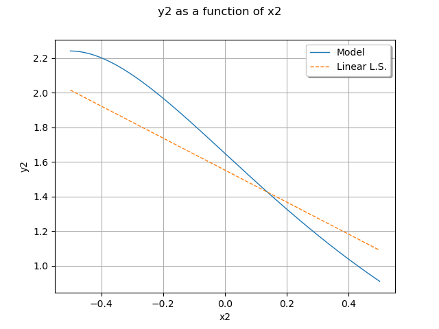
Plot the second output of our model with .
graph = ot.ParametricFunction(model, [0], [0.5]).getMarginal(1).draw(-0.5, 0.5)
graph.setLegends(["Model"])
curve = (
    ot.ParametricFunction(responseSurface, [0], [0.5])
    .getMarginal(1)
    .draw(-0.5, 0.5)
    .getDrawable(0)
)
curve.setLineStyle("dashed")
curve.setLegend("Linear L.S.")
graph.add(curve)
graph.setLegendPosition("topright")
graph.setColors(ot.Drawable.BuildDefaultPalette(2))
view = viewer.View(graph)
plt.show()

 OpenTURNS