Maximum Likelihood Principle
This method deals with the parametric modeling of a probability
distribution for a random vector
 . The appropriate
probability distribution is found by using a sample of data
. The appropriate
probability distribution is found by using a sample of data
 . Such an approach
can be described in two steps as follows:
. Such an approach
can be described in two steps as follows:
Choose a probability distribution (e.g. the Normal distribution, or any other distribution available),
Find the parameter values
 that characterize the
probability distribution (e.g. the mean and standard deviation for
the Normal distribution) which best describes the sample
.
that characterize the
probability distribution (e.g. the mean and standard deviation for
the Normal distribution) which best describes the sample
.
The maximum likelihood method is used for the second step.
This method is restricted to the
case where  and continuous probability distributions.
Please note therefore that
and continuous probability distributions.
Please note therefore that  in the following
text. The maximum likelihood estimate (MLE) of is
defined as the value of which maximizes the
likelihood function
in the following
text. The maximum likelihood estimate (MLE) of is
defined as the value of which maximizes the
likelihood function  :
:

Given that  is a sample of
independent identically distributed (i.i.d) observations,
is a sample of
independent identically distributed (i.i.d) observations,
 represents the
probability of observing such a sample assuming that they are taken from
a probability distribution with parameters . In
concrete terms, the likelihood
is calculated as
follows:
represents the
probability of observing such a sample assuming that they are taken from
a probability distribution with parameters . In
concrete terms, the likelihood
is calculated as
follows:

if the distribution is continuous, with density
 .
.
For example, if we suppose that  is a Gaussian distribution
with parameters
is a Gaussian distribution
with parameters  (i.e. the mean
and standard deviation),
(i.e. the mean
and standard deviation),
![\begin{aligned}
L\left(x_1,\ldots, x_N, \vect{\theta}\right) &=& \prod_{j=1}^{N} \frac{1}{\sigma \sqrt{2\pi}} \exp \left[ -\frac{1}{2} \left( \frac{x_j-\mu}{\sigma} \right)^2 \right] \\
&=& \frac{1}{\sigma^N (2\pi)^{N/2}} \exp \left[ -\frac{1}{2\sigma^2} \sum_{j=1}^N \left( x_j-\mu \right)^2 \right]
\end{aligned}](data:image/svg+xml;base64,PD94bWwgdmVyc2lvbj0nMS4wJyBlbmNvZGluZz0nVVRGLTgnPz4KPCEtLSBUaGlzIGZpbGUgd2FzIGdlbmVyYXRlZCBieSBkdmlzdmdtIDMuMS4yIC0tPgo8c3ZnIHZlcnNpb249JzEuMScgeG1sbnM9J2h0dHA6Ly93d3cudzMub3JnLzIwMDAvc3ZnJyB4bWxuczp4bGluaz0naHR0cDovL3d3dy53My5vcmcvMTk5OS94bGluaycgd2lkdGg9JzI5NC40NzE2MDZwdCcgaGVpZ2h0PSc3OC40NjEzMzJwdCcgdmlld0JveD0nNDcuMDM1NjgzIC03OS42NTY4NDYgMjk0LjQ3MTYwNiA3OC40NjEzMzInPgo8ZGVmcz4KPHBhdGggaWQ9J2cyLTAnIGQ9J003Ljg3ODQ1Ni0yLjc0OTY4OUM4LjA4MTY5NC0yLjc0OTY4OSA4LjI5Njg4Ny0yLjc0OTY4OSA4LjI5Njg4Ny0yLjk4ODc5MlM4LjA4MTY5NC0zLjIyNzg5NSA3Ljg3ODQ1Ni0zLjIyNzg5NUgxLjQxMDcxQzEuMjA3NDcyLTMuMjI3ODk1IC45OTIyNzktMy4yMjc4OTUgLjk5MjI3OS0yLjk4ODc5MlMxLjIwNzQ3Mi0yLjc0OTY4OSAxLjQxMDcxLTIuNzQ5Njg5SDcuODc4NDU2WicvPgo8cGF0aCBpZD0nZzItMTEyJyBkPSdNNC42NTA1NiAxMC4yMjE2NjlMMi41NDY0NTEgNS41NzExMDhDMi40NjI3NjUgNS4zNzk4MjYgMi40MDI5ODkgNS4zNzk4MjYgMi4zNjcxMjMgNS4zNzk4MjZDMi4zNTUxNjggNS4zNzk4MjYgMi4yOTUzOTIgNS4zNzk4MjYgMi4xNjM4ODUgNS40NzU0NjdMMS4wMjgxNDQgNi4zMzYyMzlDLjg3MjcyNyA2LjQ1NTc5MSAuODcyNzI3IDYuNDkxNjU2IC44NzI3MjcgNi41Mjc1MjJDLjg3MjcyNyA2LjU4NzI5OCAuOTA4NTkzIDYuNjU5MDI5IC45OTIyNzkgNi42NTkwMjlDMS4wNjQwMSA2LjY1OTAyOSAxLjI2NzI0OCA2LjQ5MTY1NiAxLjM5ODc1NSA2LjM5NjAxNUMxLjQ3MDQ4NiA2LjMzNjIzOSAxLjY0OTgxMyA2LjIwNDczMiAxLjc4MTMyIDYuMTA5MDkxTDQuMTM2NDg4IDExLjI4NTY3OUM0LjIyMDE3NCAxMS40NzY5NjEgNC4yNzk5NSAxMS40NzY5NjEgNC4zODc1NDcgMTEuNDc2OTYxQzQuNTY2ODc0IDExLjQ3Njk2MSA0LjYwMjc0IDExLjQwNTIzIDQuNjg2NDI2IDExLjIzNzg1OEwxMC4xMTQwNzIgMEMxMC4xOTc3NTgtLjE2NzM3MiAxMC4xOTc3NTgtLjIxNTE5MyAxMC4xOTc3NTgtLjIzOTEwM0MxMC4xOTc3NTgtLjM1ODY1NSAxMC4xMDIxMTctLjQ3ODIwNyA5Ljk1ODY1NS0uNDc4MjA3QzkuODYzMDE0LS40NzgyMDcgOS43NzkzMjgtLjQxODQzMSA5LjY4MzY4Ni0uMjI3MTQ4TDQuNjUwNTYgMTAuMjIxNjY5WicvPgo8cGF0aCBpZD0nZzEtMTgnIGQ9J004LjM2ODYxOCAyOC4wODI2OUM4LjM2ODYxOCAyOC4wMzQ4NjkgOC4zNDQ3MDcgMjguMDEwOTU5IDguMzIwNzk3IDI3Ljk3NTA5M0M3Ljg3ODQ1NiAyNy41MzI3NTIgNy4wNzc0NiAyNi43MzE3NTYgNi4yNzY0NjMgMjUuNDQwNTk4QzQuMzUxNjgxIDIyLjM1NjE2NCAzLjQ3ODk1NCAxOC40NzA3MzUgMy40Nzg5NTQgMTMuODY3OTk1QzMuNDc4OTU0IDEwLjY1MjA1NSAzLjkwOTM0IDYuNTAzNjExIDUuODgxOTQzIDIuOTQwOTcxQzYuODI2NDAxIDEuMjQzMzM3IDcuODA2NzI1IC4yNjMwMTQgOC4zMzI3NTItLjI2MzAxNEM4LjM2ODYxOC0uMjk4ODc5IDguMzY4NjE4LS4zMjI3OSA4LjM2ODYxOC0uMzU4NjU1QzguMzY4NjE4LS40NzgyMDcgOC4yODQ5MzItLjQ3ODIwNyA4LjExNzU1OS0uNDc4MjA3UzcuOTI2Mjc2LS40NzgyMDcgNy43NDY5NDktLjI5ODg3OUMzLjc0MTk2OCAzLjM0NzQ0NyAyLjQ4NjY3NSA4LjgyMjkxNCAyLjQ4NjY3NSAxMy44NTYwNEMyLjQ4NjY3NSAxOC41NTQ0MjEgMy41NjI2NCAyMy4yODg2NjcgNi41OTkyNTMgMjYuODYzMjYzQzYuODM4MzU2IDI3LjEzODIzMiA3LjI5MjY1MyAyNy42MjgzOTQgNy43ODI4MTQgMjguMDU4NzhDNy45MjYyNzYgMjguMjAyMjQyIDcuOTUwMTg3IDI4LjIwMjI0MiA4LjExNzU1OSAyOC4yMDIyNDJTOC4zNjg2MTggMjguMjAyMjQyIDguMzY4NjE4IDI4LjA4MjY5WicvPgo8cGF0aCBpZD0nZzEtMTknIGQ9J002LjMwMDM3NCAxMy44Njc5OTVDNi4zMDAzNzQgOS4xNjk2MTQgNS4yMjQ0MDggNC40MzUzNjcgMi4xODc3OTYgLjg2MDc3MkMxLjk0ODY5MiAuNTg1ODAzIDEuNDk0Mzk2IC4wOTU2NDEgMS4wMDQyMzQtLjMzNDc0NUMuODYwNzcyLS40NzgyMDcgLjgzNjg2Mi0uNDc4MjA3IC42Njk0ODktLjQ3ODIwN0MuNTI2MDI3LS40NzgyMDcgLjQxODQzMS0uNDc4MjA3IC40MTg0MzEtLjM1ODY1NUMuNDE4NDMxLS4zMTA4MzQgLjQ2NjI1Mi0uMjYzMDE0IC40OTAxNjItLjIzOTEwM0MuOTA4NTkzIC4xOTEyODMgMS43MDk1ODkgLjk5MjI3OSAyLjUxMDU4NSAyLjI4MzQzN0M0LjQzNTM2NyA1LjM2Nzg3IDUuMzA4MDk1IDkuMjUzMyA1LjMwODA5NSAxMy44NTYwNEM1LjMwODA5NSAxNy4wNzE5OCA0Ljg3NzcwOSAyMS4yMjA0MjMgMi45MDUxMDYgMjQuNzgzMDY0QzEuOTYwNjQ4IDI2LjQ4MDY5NyAuOTY4MzY5IDI3LjQ3Mjk3NiAuNDY2MjUyIDI3Ljk3NTA5M0MuNDQyMzQxIDI4LjAxMDk1OSAuNDE4NDMxIDI4LjA0NjgyNCAuNDE4NDMxIDI4LjA4MjY5Qy40MTg0MzEgMjguMjAyMjQyIC41MjYwMjcgMjguMjAyMjQyIC42Njk0ODkgMjguMjAyMjQyQy44MzY4NjIgMjguMjAyMjQyIC44NjA3NzIgMjguMjAyMjQyIDEuMDQwMSAyOC4wMjI5MTRDNS4wNDUwODEgMjQuMzc2NTg4IDYuMzAwMzc0IDE4LjkwMTEyMSA2LjMwMDM3NCAxMy44Njc5OTVaJy8+CjxwYXRoIGlkPSdnMS0zNCcgZD0nTTMuMjg3NjcxIDM1LjM3NTM0Mkg2LjgyNjQwMVYzNC42MzQxMjJINC4wMjg4OTJWLjI2MzAxNEg2LjgyNjQwMVYtLjQ3ODIwN0gzLjI4NzY3MVYzNS4zNzUzNDJaJy8+CjxwYXRoIGlkPSdnMS0zNScgZD0nTTIuOTI5MDE2IDM0LjYzNDEyMkguMTMxNTA3VjM1LjM3NTM0MkgzLjY3MDIzN1YtLjQ3ODIwN0guMTMxNTA3Vi4yNjMwMTRIMi45MjkwMTZWMzQuNjM0MTIyWicvPgo8cGF0aCBpZD0nZzEtODgnIGQ9J00xNS4xMzUyNDMgMTYuNzM3MjM1TDE2LjU4MTgxOCAxMi45MTE1ODJIMTYuMjgyOTM5QzE1LjgxNjY4NyAxNC4xNTQ5MTkgMTQuNTQ5NDQgMTQuOTY3ODcgMTMuMTc0NTk1IDE1LjMyNjUyNkMxMi45MjM1MzcgMTUuMzg2MzAxIDExLjc1MTkzIDE1LjY5NzEzNiA5LjQ1NjUzOCAxNS42OTcxMzZIMi4yNDc1NzJMOC4zMzI3NTIgOC41NTk5QzguNDE2NDM4IDguNDY0MjU5IDguNDQwMzQ5IDguNDI4Mzk0IDguNDQwMzQ5IDguMzY4NjE4QzguNDQwMzQ5IDguMzQ0NzA3IDguNDQwMzQ5IDguMzA4ODQyIDguMzU2NjYzIDguMTg5MjlMMi43ODU1NTQgLjU3Mzg0OEg5LjMzNjk4NkMxMC45Mzg5NzkgLjU3Mzg0OCAxMi4wMjY4OTkgLjc0MTIyIDEyLjEzNDQ5NiAuNzY1MTMxQzEyLjc4MDA3NSAuODYwNzcyIDEzLjgyMDE3NCAxLjA2NDAxIDE0Ljc2NDYzMyAxLjY2MTc2OEMxNS4wNjM1MTIgMS44NTMwNTEgMTUuODc2NDYzIDIuMzkxMDM0IDE2LjI4MjkzOSAzLjM1OTQwMkgxNi41ODE4MThMMTUuMTM1MjQzIDBIMS4wMDQyMzRDLjcyOTI2NSAwIC43MTczMSAuMDExOTU1IC42ODE0NDUgLjA4MzY4NkMuNjY5NDg5IC4xMTk1NTIgLjY2OTQ4OSAuMzQ2NyAuNjY5NDg5IC40NzgyMDdMNi45OTM3NzMgOS4xMzM3NDhMLjgwMDk5NiAxNi4zOTA1MzVDLjY4MTQ0NSAxNi41MzM5OTggLjY4MTQ0NSAxNi41OTM3NzMgLjY4MTQ0NSAxNi42MDU3MjlDLjY4MTQ0NSAxNi43MzcyMzUgLjc4OTA0MSAxNi43MzcyMzUgMS4wMDQyMzQgMTYuNzM3MjM1SDE1LjEzNTI0M1onLz4KPHBhdGggaWQ9J2cxLTg5JyBkPSdNMTQuNTk3MjYgMTYuNzM3MjM1VjE2LjA5MTY1NkMxMy4wMDcyMjMgMTYuMDkxNjU2IDEyLjYzNjYxMyAxNS41NDE3MTkgMTIuNjM2NjEzIDE0Ljc3NjU4OFYxLjk2MDY0OEMxMi42MzY2MTMgMS4xODM1NjIgMTMuMDE5MTc4IC42NDU1NzkgMTQuNTk3MjYgLjY0NTU3OVYwSC42Njk0ODlWLjY0NTU3OUMyLjI1OTUyNyAuNjQ1NTc5IDIuNjMwMTM3IDEuMTk1NTE3IDIuNjMwMTM3IDEuOTYwNjQ4VjE0Ljc3NjU4OEMyLjYzMDEzNyAxNS41NTM2NzQgMi4yNDc1NzIgMTYuMDkxNjU2IC42Njk0ODkgMTYuMDkxNjU2VjE2LjczNzIzNUg2LjQxOTkyNVYxNi4wOTE2NTZDNC44Mjk4ODggMTYuMDkxNjU2IDQuNDU5Mjc4IDE1LjU0MTcxOSA0LjQ1OTI3OCAxNC43NzY1ODhWLjY0NTU3OUgxMC44MDc0NzJWMTQuNzc2NTg4QzEwLjgwNzQ3MiAxNS41NTM2NzQgMTAuNDI0OTA3IDE2LjA5MTY1NiA4Ljg0NjgyNCAxNi4wOTE2NTZWMTYuNzM3MjM1SDE0LjU5NzI2WicvPgo8cGF0aCBpZD0nZzAtMTgnIGQ9J002LjUzOTQ3Ny01Ljg1ODAzMkM2LjUzOTQ3Ny03Ljk2MjE0MiA1LjI5NjEzOS04LjM5MjUyOCA0LjU2Njg3NC04LjM5MjUyOEMzLjYyMjQxNi04LjM5MjUyOCAyLjQyNjg5OS03Ljc3MDg1OSAxLjUzMDI2Mi02LjE0NDk1NkMuOTIwNTQ4LTUuMDIxMTcxIC41NDk5MzgtMy4zOTUyNjggLjU0OTkzOC0yLjQyNjg5OUMuNTQ5OTM4LS42OTM0IDEuNDU4NTMxIC4wOTU2NDEgMi41MzQ0OTYgLjA5NTY0MUMzLjMzNTQ5MiAuMDk1NjQxIDQuMzg3NTQ3LS4zNzA2MSA1LjIxMjQ1My0xLjU5MDAzN0M2LjIxNjY4Ny0zLjA2MDUyMyA2LjUzOTQ3Ny00Ljk2MTM5NSA2LjUzOTQ3Ny01Ljg1ODAzMlpNMi4zNjcxMjMtNC40MzUzNjdDMi41MzQ0OTYtNS4xMjg3NjcgMi44NDUzMy02LjIxNjY4NyAzLjIwMzk4NS02LjgzODM1NkMzLjQ3ODk1NC03LjMyODUxOCAzLjk2OTExNi03Ljk2MjE0MiA0LjU0Mjk2NC03Ljk2MjE0MkM1LjA0NTA4MS03Ljk2MjE0MiA1LjI2MDI3NC03LjQzNjExNSA1LjI2MDI3NC02LjczMDc2QzUuMjYwMjc0LTUuOTc3NTg0IDQuOTk3MjYtNC45Mzc0ODQgNC44NjU3NTMtNC40MzUzNjdIMi4zNjcxMjNaTTQuNzIyMjkxLTMuODYxNTE5QzMuOTgxMDcxLS42NTc1MzQgMi45NzY4MzctLjMzNDc0NSAyLjU1ODQwNi0uMzM0NzQ1QzIuMzkxMDM0LS4zMzQ3NDUgMi4xMzk5NzUtLjM4MjU2NSAxLjk3MjYwMy0uNzUzMTc2QzEuODI5MTQxLTEuMDc1OTY1IDEuODI5MTQxLTEuNTQyMjE3IDEuODI5MTQxLTEuNTU0MTcyQzEuODI5MTQxLTIuMjM1NjE2IDIuMDkyMTU0LTMuMzQ3NDQ3IDIuMjIzNjYxLTMuODYxNTE5SDQuNzIyMjkxWicvPgo8cGF0aCBpZD0nZzMtNjEnIGQ9J00zLjcwNjEwMi01LjY0MjgzOUMzLjc1MzkyMy01Ljc1NDQyMSAzLjc1MzkyMy01Ljc3MDM2MSAzLjc1MzkyMy01Ljc5NDI3MUMzLjc1MzkyMy01Ljg5Nzg4MyAzLjY3NDIyMi01Ljk3NzU4NCAzLjU3MDYxLTUuOTc3NTg0QzMuNDQzMDg4LTUuOTc3NTg0IDMuNDExMjA4LTUuODgxOTQzIDMuMzc5MzI4LTUuODAyMjQyTC41MTgwNTcgMS42NTc3ODNDLjQ3MDIzNyAxLjc2OTM2NSAuNDcwMjM3IDEuNzg1MzA1IC40NzAyMzcgMS44MDkyMTVDLjQ3MDIzNyAxLjkxMjgyNyAuNTQ5OTM4IDEuOTkyNTI4IC42NTM1NDkgMS45OTI1MjhDLjc4MTA3MSAxLjk5MjUyOCAuODEyOTUxIDEuODk2ODg3IC44NDQ4MzIgMS44MTcxODZMMy43MDYxMDItNS42NDI4MzlaJy8+CjxwYXRoIGlkPSdnMy03OCcgZD0nTTYuMzEyMzI5LTQuNTc0ODQ0QzYuNDA3OTctNC45NjUzOCA2LjU4MzMxMy01LjE1NjY2MyA3LjE1NzE2MS01LjE4MDU3M0M3LjIzNjg2Mi01LjE4MDU3MyA3LjMwMDYyMy01LjIyODM5NCA3LjMwMDYyMy01LjMzMjAwNUM3LjMwMDYyMy01LjM3OTgyNiA3LjI2MDc3Mi01LjQ0MzU4NyA3LjE4MTA3MS01LjQ0MzU4N0M3LjEyNTI4LTUuNDQzNTg3IDYuOTczODQ4LTUuNDE5Njc2IDYuMzg0MDYtNS40MTk2NzZDNS43NDY0NTEtNS40MTk2NzYgNS42NDI4MzktNS40NDM1ODcgNS41NzExMDgtNS40NDM1ODdDNS40NDM1ODctNS40NDM1ODcgNS40MTk2NzYtNS4zNTU5MTUgNS40MTk2NzYtNS4yOTIxNTRDNS40MTk2NzYtNS4xODg1NDMgNS41MjMyODgtNS4xODA1NzMgNS41OTUwMTktNS4xODA1NzNDNi4wODExOTYtNS4xNjQ2MzMgNi4wODExOTYtNC45NDk0NCA2LjA4MTE5Ni00LjgzNzg1OEM2LjA4MTE5Ni00Ljc5ODAwNyA2LjA4MTE5Ni00Ljc1ODE1NyA2LjA0OTMxNS00LjYzMDYzNUw1LjE3MjYwMy0xLjEzOTcyNkwzLjI1MTgwNi01LjMwMDEyNUMzLjE4ODA0NS01LjQ0MzU4NyAzLjE3MjEwNS01LjQ0MzU4NyAyLjk4MDgyMi01LjQ0MzU4N0gxLjk0NDcwN0MxLjgwMTI0NS01LjQ0MzU4NyAxLjY5NzYzNC01LjQ0MzU4NyAxLjY5NzYzNC01LjI5MjE1NEMxLjY5NzYzNC01LjE4MDU3MyAxLjc5MzI3NS01LjE4MDU3MyAxLjk2MDY0OC01LjE4MDU3M0MyLjAyNDQwOC01LjE4MDU3MyAyLjI2MzUxMi01LjE4MDU3MyAyLjQ0NjgyNC01LjEzMjc1MkwxLjM3ODgyOS0uODUyODAyQzEuMjgzMTg4LS40NTQyOTYgMS4wNzU5NjUtLjI3ODk1NCAuNTQxOTY4LS4yNjMwMTRDLjQ5NDE0Ny0uMjYzMDE0IC4zOTg1MDYtLjI1NTA0NCAuMzk4NTA2LS4xMTE1ODJDLjM5ODUwNi0uMDYzNzYxIC40MzgzNTYgMCAuNTE4MDU3IDBDLjU0OTkzOCAwIC43MzMyNS0uMDIzOTEgMS4zMDcwOTgtLjAyMzkxQzEuOTM2NzM3LS4wMjM5MSAyLjA1NjI4OSAwIDIuMTI4MDIgMEMyLjE1OTkgMCAyLjI3OTQ1MiAwIDIuMjc5NDUyLS4xNTE0MzJDMi4yNzk0NTItLjI0NzA3MyAyLjE5MTc4MS0uMjYzMDE0IDIuMTM1OTktLjI2MzAxNEMxLjg0OTA2Ni0uMjcwOTg0IDEuNjA5OTYzLS4zMTg4MDQgMS42MDk5NjMtLjU5Nzc1OEMxLjYwOTk2My0uNjM3NjA5IDEuNjMzODczLS43NDkxOTEgMS42MzM4NzMtLjc1NzE2MUwyLjY3Nzk1OC00LjkxNzU1OUgyLjY4NTkyOEw0LjkwMTYxOS0uMTQzNDYyQzQuOTU3NDEtLjAxNTk0IDQuOTY1MzggMCA1LjA1MzA1MSAwQzUuMTY0NjMzIDAgNS4xNzI2MDMtLjAzMTg4IDUuMjA0NDgzLS4xNjczNzJMNi4zMTIzMjktNC41NzQ4NDRaJy8+CjxwYXRoIGlkPSdnMy0xMDYnIGQ9J00zLjI5MTY1Ni00Ljk3MzM1QzMuMjkxNjU2LTUuMTI0NzgyIDMuMTcyMTA1LTUuMjc2MjE0IDIuOTgwODIyLTUuMjc2MjE0QzIuNzQxNzE5LTUuMjc2MjE0IDIuNTM0NDk2LTUuMDUzMDUxIDIuNTM0NDk2LTQuODQ1ODI4QzIuNTM0NDk2LTQuNjk0Mzk2IDIuNjU0MDQ3LTQuNTQyOTY0IDIuODQ1MzMtNC41NDI5NjRDMy4wODQ0MzMtNC41NDI5NjQgMy4yOTE2NTYtNC43NjYxMjcgMy4yOTE2NTYtNC45NzMzNVpNMS42MjU5MDMgLjM5ODUwNkMxLjUwNjM1MSAuODg0NjgyIDEuMTE1ODE2IDEuNDAyNzQgLjYyOTYzOSAxLjQwMjc0Qy41MDIxMTcgMS40MDI3NCAuMzgyNTY1IDEuMzcwODU5IC4zNjY2MjUgMS4zNjI4ODlDLjYxMzY5OSAxLjI0MzMzNyAuNjQ1NTc5IDEuMDI4MTQ0IC42NDU1NzkgLjk1NjQxM0MuNjQ1NTc5IC43NjUxMzEgLjUwMjExNyAuNjYxNTE5IC4zMzQ3NDUgLjY2MTUxOUMuMTAzNjExIC42NjE1MTktLjExMTU4MiAuODYwNzcyLS4xMTE1ODIgMS4xMjM3ODZDLS4xMTE1ODIgMS40MjY2NSAuMTgzMzEzIDEuNjI1OTAzIC42Mzc2MDkgMS42MjU5MDNDMS4xMjM3ODYgMS42MjU5MDMgMi4wMDA0OTggMS4zMjMwMzkgMi4yMzk2MDEgLjM2NjYyNUwyLjk1NjkxMi0yLjQ4NjY3NUMyLjk4MDgyMi0yLjU4MjMxNiAyLjk5Njc2Mi0yLjY0NjA3NyAyLjk5Njc2Mi0yLjc2NTYyOUMyLjk5Njc2Mi0zLjIwMzk4NSAyLjY0NjA3Ny0zLjUxNDgxOSAyLjE4MzgxMS0zLjUxNDgxOUMxLjMzODk3OS0zLjUxNDgxOSAuODQ0ODMyLTIuMzk5MDA0IC44NDQ4MzItMi4yOTUzOTJDLjg0NDgzMi0yLjIyMzY2MSAuOTAwNjIzLTIuMTkxNzgxIC45NjQzODQtMi4xOTE3ODFDMS4wNTIwNTUtMi4xOTE3ODEgMS4wNjAwMjUtMi4yMTU2OTEgMS4xMTU4MTYtMi4zMzUyNDNDMS4zNTQ5MTktMi44ODUxODEgMS43NjEzOTUtMy4yOTE2NTYgMi4xNTk5LTMuMjkxNjU2QzIuMzI3MjczLTMuMjkxNjU2IDIuNDIyOTE0LTMuMTgwMDc1IDIuNDIyOTE0LTIuOTE3MDYxQzIuNDIyOTE0LTIuODA1NDc5IDIuMzk5MDA0LTIuNjkzODk4IDIuMzc1MDkzLTIuNTgyMzE2TDEuNjI1OTAzIC4zOTg1MDZaJy8+CjxwYXRoIGlkPSdnNS00OScgZD0nTTIuNTAyNjE1LTUuMDc2OTYxQzIuNTAyNjE1LTUuMjkyMTU0IDIuNDg2Njc1LTUuMzAwMTI1IDIuMjcxNDgyLTUuMzAwMTI1QzEuOTQ0NzA3LTQuOTgxMzIgMS41MjIyOTEtNC43OTAwMzcgLjc2NTEzMS00Ljc5MDAzN1YtNC41MjcwMjRDLjk4MDMyNC00LjUyNzAyNCAxLjQxMDcxLTQuNTI3MDI0IDEuODcyOTc2LTQuNzQyMjE3Vi0uNjUzNTQ5QzEuODcyOTc2LS4zNTg2NTUgMS44NDkwNjYtLjI2MzAxNCAxLjA5MTkwNS0uMjYzMDE0SC44MTI5NTFWMEMxLjEzOTcyNi0uMDIzOTEgMS44MjUxNTYtLjAyMzkxIDIuMTgzODExLS4wMjM5MVMzLjIzNTg2Ni0uMDIzOTEgMy41NjI2NCAwVi0uMjYzMDE0SDMuMjgzNjg2QzIuNTI2NTI2LS4yNjMwMTQgMi41MDI2MTUtLjM1ODY1NSAyLjUwMjYxNS0uNjUzNTQ5Vi01LjA3Njk2MVonLz4KPHBhdGggaWQ9J2c1LTUwJyBkPSdNMi4yNDc1NzItMS42MjU5MDNDMi4zNzUwOTMtMS43NDU0NTUgMi43MDk4MzgtMi4wMDg0NjggMi44MzczNi0yLjEyMDA1QzMuMzMxNTA3LTIuNTc0MzQ2IDMuODAxNzQzLTMuMDEyNzAyIDMuODAxNzQzLTMuNzM3OTgzQzMuODAxNzQzLTQuNjg2NDI2IDMuMDA0NzMyLTUuMzAwMTI1IDIuMDA4NDY4LTUuMzAwMTI1QzEuMDUyMDU1LTUuMzAwMTI1IC40MjI0MTYtNC41NzQ4NDQgLjQyMjQxNi0zLjg2NTUwNEMuNDIyNDE2LTMuNDc0OTY5IC43MzMyNS0zLjQxOTE3OCAuODQ0ODMyLTMuNDE5MTc4QzEuMDEyMjA0LTMuNDE5MTc4IDEuMjU5Mjc4LTMuNTM4NzMgMS4yNTkyNzgtMy44NDE1OTRDMS4yNTkyNzgtNC4yNTYwNCAuODYwNzcyLTQuMjU2MDQgLjc2NTEzMS00LjI1NjA0Qy45OTYyNjQtNC44Mzc4NTggMS41MzAyNjItNS4wMzcxMTEgMS45MjA3OTctNS4wMzcxMTFDMi42NjIwMTctNS4wMzcxMTEgMy4wNDQ1ODMtNC40MDc0NzIgMy4wNDQ1ODMtMy43Mzc5ODNDMy4wNDQ1ODMtMi45MDkwOTEgMi40NjI3NjUtMi4zMDMzNjIgMS41MjIyOTEtMS4zMzg5NzlMLjUxODA1Ny0uMzAyODY0Qy40MjI0MTYtLjIxNTE5MyAuNDIyNDE2LS4xOTkyNTMgLjQyMjQxNiAwSDMuNTcwNjFMMy44MDE3NDMtMS40MjY2NUgzLjU1NDY3QzMuNTMwNzYtMS4yNjcyNDggMy40NjY5OTktLjg2ODc0MiAzLjM3MTM1Ny0uNzE3MzFDMy4zMjM1MzctLjY1MzU0OSAyLjcxNzgwOC0uNjUzNTQ5IDIuNTkwMjg2LS42NTM1NDlIMS4xNzE2MDZMMi4yNDc1NzItMS42MjU5MDNaJy8+CjxwYXRoIGlkPSdnNS02MScgZD0nTTUuODI2MTUyLTIuNjU0MDQ3QzUuOTQ1NzA0LTIuNjU0MDQ3IDYuMTA1MTA2LTIuNjU0MDQ3IDYuMTA1MTA2LTIuODM3MzZTNS45MTM4MjMtMy4wMjA2NzIgNS43OTQyNzEtMy4wMjA2NzJILjc4MTA3MUMuNjYxNTE5LTMuMDIwNjcyIC40NzAyMzctMy4wMjA2NzIgLjQ3MDIzNy0yLjgzNzM2Uy42Mjk2MzktMi42NTQwNDcgLjc0OTE5MS0yLjY1NDA0N0g1LjgyNjE1MlpNNS43OTQyNzEtLjk2NDM4NEM1LjkxMzgyMy0uOTY0Mzg0IDYuMTA1MTA2LS45NjQzODQgNi4xMDUxMDYtMS4xNDc2OTZTNS45NDU3MDQtMS4zMzEwMDkgNS44MjYxNTItMS4zMzEwMDlILjc0OTE5MUMuNjI5NjM5LTEuMzMxMDA5IC40NzAyMzctMS4zMzEwMDkgLjQ3MDIzNy0xLjE0NzY5NlMuNjYxNTE5LS45NjQzODQgLjc4MTA3MS0uOTY0Mzg0SDUuNzk0MjcxWicvPgo8cGF0aCBpZD0nZzYtNDAnIGQ9J00zLjg4NTQzIDIuOTA1MTA2QzMuODg1NDMgMi44NjkyNCAzLjg4NTQzIDIuODQ1MzMgMy42ODIxOTIgMi42NDIwOTJDMi40ODY2NzUgMS40MzQ2MiAxLjgxNzE4Ni0uNTM3OTgzIDEuODE3MTg2LTIuOTc2ODM3QzEuODE3MTg2LTUuMjk2MTM5IDIuMzc5MDc4LTcuMjkyNjUzIDMuNzY1ODc4LTguNzAzMzYyQzMuODg1NDMtOC44MTA5NTkgMy44ODU0My04LjgzNDg2OSAzLjg4NTQzLTguODcwNzM1QzMuODg1NDMtOC45NDI0NjYgMy44MjU2NTQtOC45NjYzNzYgMy43Nzc4MzMtOC45NjYzNzZDMy42MjI0MTYtOC45NjYzNzYgMi42NDIwOTItOC4xMDU2MDQgMi4wNTYyODktNi45MzM5OThDMS40NDY1NzUtNS43MjY1MjYgMS4xNzE2MDYtNC40NDczMjMgMS4xNzE2MDYtMi45NzY4MzdDMS4xNzE2MDYtMS45MTI4MjcgMS4zMzg5NzktLjQ5MDE2MiAxLjk2MDY0OCAuNzg5MDQxQzIuNjY2MDAyIDIuMjIzNjYxIDMuNjQ2MzI2IDMuMDAwNzQ3IDMuNzc3ODMzIDMuMDAwNzQ3QzMuODI1NjU0IDMuMDAwNzQ3IDMuODg1NDMgMi45NzY4MzcgMy44ODU0MyAyLjkwNTEwNlonLz4KPHBhdGggaWQ9J2c2LTQxJyBkPSdNMy4zNzEzNTctMi45NzY4MzdDMy4zNzEzNTctMy44ODU0MyAzLjI1MTgwNi01LjM2Nzg3IDIuNTgyMzE2LTYuNzU0NjdDMS44NzY5NjEtOC4xODkyOSAuODk2NjM4LTguOTY2Mzc2IC43NjUxMzEtOC45NjYzNzZDLjcxNzMxLTguOTY2Mzc2IC42NTc1MzQtOC45NDI0NjYgLjY1NzUzNC04Ljg3MDczNUMuNjU3NTM0LTguODM0ODY5IC42NTc1MzQtOC44MTA5NTkgLjg2MDc3Mi04LjYwNzcyMUMyLjA1NjI4OS03LjQwMDI0OSAyLjcyNTc3OC01LjQyNzY0NiAyLjcyNTc3OC0yLjk4ODc5MkMyLjcyNTc3OC0uNjY5NDg5IDIuMTYzODg1IDEuMzI3MDI0IC43NzcwODYgMi43Mzc3MzNDLjY1NzUzNCAyLjg0NTMzIC42NTc1MzQgMi44NjkyNCAuNjU3NTM0IDIuOTA1MTA2Qy42NTc1MzQgMi45NzY4MzcgLjcxNzMxIDMuMDAwNzQ3IC43NjUxMzEgMy4wMDA3NDdDLjkyMDU0OCAzLjAwMDc0NyAxLjkwMDg3MiAyLjEzOTk3NSAyLjQ4NjY3NSAuOTY4MzY5QzMuMDk2Mzg5LS4yNTEwNTkgMy4zNzEzNTctMS41NDIyMTcgMy4zNzEzNTctMi45NzY4MzdaJy8+CjxwYXRoIGlkPSdnNi00OScgZD0nTTMuNDQzMDg4LTcuNjYzMjYzQzMuNDQzMDg4LTcuOTM4MjMyIDMuNDQzMDg4LTcuOTUwMTg3IDMuMjAzOTg1LTcuOTUwMTg3QzIuOTE3MDYxLTcuNjI3Mzk3IDIuMzE5MzAzLTcuMTg1MDU2IDEuMDg3OTItNy4xODUwNTZWLTYuODM4MzU2QzEuMzYyODg5LTYuODM4MzU2IDEuOTYwNjQ4LTYuODM4MzU2IDIuNjE4MTgyLTcuMTQ5MTkxVi0uOTIwNTQ4QzIuNjE4MTgyLS40OTAxNjIgMi41ODIzMTYtLjM0NjcgMS41MzAyNjItLjM0NjdIMS4xNTk2NTFWMEMxLjQ4MjQ0MS0uMDIzOTEgMi42NDIwOTItLjAyMzkxIDMuMDM2NjEzLS4wMjM5MVM0LjU3ODgyOS0uMDIzOTEgNC45MDE2MTkgMFYtLjM0NjdINC41MzEwMDlDMy40Nzg5NTQtLjM0NjcgMy40NDMwODgtLjQ5MDE2MiAzLjQ0MzA4OC0uOTIwNTQ4Vi03LjY2MzI2M1onLz4KPHBhdGggaWQ9J2c2LTUwJyBkPSdNNS4yNjAyNzQtMi4wMDg0NjhINC45OTcyNkM0Ljk2MTM5NS0xLjgwNTIzIDQuODY1NzUzLTEuMTQ3Njk2IDQuNzQ2MjAyLS45NTY0MTNDNC42NjI1MTYtLjg0ODgxNyAzLjk4MTA3MS0uODQ4ODE3IDMuNjIyNDE2LS44NDg4MTdIMS40MTA3MUMxLjczMzQ5OS0xLjEyMzc4NiAyLjQ2Mjc2NS0xLjg4ODkxNyAyLjc3MzU5OS0yLjE3NTg0MUM0LjU5MDc4NS0zLjg0OTU2NCA1LjI2MDI3NC00LjQ3MTIzMyA1LjI2MDI3NC01LjY1NDc5NUM1LjI2MDI3NC03LjAyOTYzOSA0LjE3MjM1NC03Ljk1MDE4NyAyLjc4NTU1NC03Ljk1MDE4N1MuNTg1ODAzLTYuNzY2NjI1IC41ODU4MDMtNS43Mzg0ODFDLjU4NTgwMy01LjEyODc2NyAxLjExMTgzMS01LjEyODc2NyAxLjE0NzY5Ni01LjEyODc2N0MxLjM5ODc1NS01LjEyODc2NyAxLjcwOTU4OS01LjMwODA5NSAxLjcwOTU4OS01LjY5MDY2QzEuNzA5NTg5LTYuMDI1NDA1IDEuNDgyNDQxLTYuMjUyNTUzIDEuMTQ3Njk2LTYuMjUyNTUzQzEuMDQwMS02LjI1MjU1MyAxLjAxNjE4OS02LjI1MjU1MyAuOTgwMzI0LTYuMjQwNTk4QzEuMjA3NDcyLTcuMDUzNTQ5IDEuODUzMDUxLTcuNjAzNDg3IDIuNjMwMTM3LTcuNjAzNDg3QzMuNjQ2MzI2LTcuNjAzNDg3IDQuMjY3OTk1LTYuNzU0NjcgNC4yNjc5OTUtNS42NTQ3OTVDNC4yNjc5OTUtNC42Mzg2MDUgMy42ODIxOTItMy43NTM5MjMgMy4wMDA3NDctMi45ODg3OTJMLjU4NTgwMy0uMjg2OTI0VjBINC45NDk0NEw1LjI2MDI3NC0yLjAwODQ2OFonLz4KPHBhdGggaWQ9J2c2LTYxJyBkPSdNOC4wNjk3MzgtMy44NzM0NzRDOC4yMzcxMTEtMy44NzM0NzQgOC40NTIzMDQtMy44NzM0NzQgOC40NTIzMDQtNC4wODg2NjdDOC40NTIzMDQtNC4zMTU4MTYgOC4yNDkwNjYtNC4zMTU4MTYgOC4wNjk3MzgtNC4zMTU4MTZIMS4wMjgxNDRDLjg2MDc3Mi00LjMxNTgxNiAuNjQ1NTc5LTQuMzE1ODE2IC42NDU1NzktNC4xMDA2MjNDLjY0NTU3OS0zLjg3MzQ3NCAuODQ4ODE3LTMuODczNDc0IDEuMDI4MTQ0LTMuODczNDc0SDguMDY5NzM4Wk04LjA2OTczOC0xLjY0OTgxM0M4LjIzNzExMS0xLjY0OTgxMyA4LjQ1MjMwNC0xLjY0OTgxMyA4LjQ1MjMwNC0xLjg2NTAwNkM4LjQ1MjMwNC0yLjA5MjE1NCA4LjI0OTA2Ni0yLjA5MjE1NCA4LjA2OTczOC0yLjA5MjE1NEgxLjAyODE0NEMuODYwNzcyLTIuMDkyMTU0IC42NDU1NzktMi4wOTIxNTQgLjY0NTU3OS0xLjg3Njk2MUMuNjQ1NTc5LTEuNjQ5ODEzIC44NDg4MTctMS42NDk4MTMgMS4wMjgxNDQtMS42NDk4MTNIOC4wNjk3MzhaJy8+CjxwYXRoIGlkPSdnNi0xMDEnIGQ9J000LjU3ODgyOS0yLjc3MzU5OUM0Ljg0MTg0My0yLjc3MzU5OSA0Ljg2NTc1My0yLjc3MzU5OSA0Ljg2NTc1My0zLjAwMDc0N0M0Ljg2NTc1My00LjIwODIxOSA0LjIyMDE3NC01LjMzMjAwNSAyLjc3MzU5OS01LjMzMjAwNUMxLjQxMDcxLTUuMzMyMDA1IC4zNTg2NTUtNC4xMDA2MjMgLjM1ODY1NS0yLjYxODE4MkMuMzU4NjU1LTEuMDQwMSAxLjU3ODA4MiAuMTE5NTUyIDIuOTA1MTA2IC4xMTk1NTJDNC4zMjc3NzEgLjExOTU1MiA0Ljg2NTc1My0xLjE3MTYwNiA0Ljg2NTc1My0xLjQyMjY2NUM0Ljg2NTc1My0xLjQ5NDM5NiA0LjgwNTk3OC0xLjU0MjIxNyA0LjczNDI0Ny0xLjU0MjIxN0M0LjYzODYwNS0xLjU0MjIxNyA0LjYxNDY5NS0xLjQ4MjQ0MSA0LjU5MDc4NS0xLjQyMjY2NUM0LjI3OTk1LS40MTg0MzEgMy40Nzg5NTQtLjE0MzQ2MiAyLjk3NjgzNy0uMTQzNDYyUzEuMjY3MjQ4LS40NzgyMDcgMS4yNjcyNDgtMi41NDY0NTFWLTIuNzczNTk5SDQuNTc4ODI5Wk0xLjI3OTIwMy0zLjAwMDc0N0MxLjM3NDg0NC00Ljg3NzcwOSAyLjQyNjg5OS01LjA5MjkwMiAyLjc2MTY0NC01LjA5MjkwMkM0LjA0MDg0Ny01LjA5MjkwMiA0LjExMjU3OC0zLjQwNzIyMyA0LjEyNDUzMy0zLjAwMDc0N0gxLjI3OTIwM1onLz4KPHBhdGggaWQ9J2c2LTExMicgZD0nTTIuOTI5MDE2IDEuOTcyNjAzQzIuMTYzODg1IDEuOTcyNjAzIDIuMDIwNDIzIDEuOTcyNjAzIDIuMDIwNDIzIDEuNDM0NjJWLS42NDU1NzlDMi4yMzU2MTYtLjM0NjcgMi43MjU3NzggLjExOTU1MiAzLjQ5MDkwOSAuMTE5NTUyQzQuODY1NzUzIC4xMTk1NTIgNi4wNzMyMjUtMS4wNDAxIDYuMDczMjI1LTIuNTgyMzE2QzYuMDczMjI1LTQuMTAwNjIzIDQuOTQ5NDQtNS4yNzIyMjkgMy42NDYzMjYtNS4yNzIyMjlDMi41OTQyNzEtNS4yNzIyMjkgMi4wMzIzNzktNC41MTkwNTQgMS45OTY1MTMtNC40NzEyMzNWLTUuMjcyMjI5TC4zMzQ3NDUtNS4xNDA3MjJWLTQuNzk0MDIyQzEuMTcxNjA2LTQuNzk0MDIyIDEuMjQzMzM3LTQuNzEwMzM2IDEuMjQzMzM3LTQuMTg0MzA5VjEuNDM0NjJDMS4yNDMzMzcgMS45NzI2MDMgMS4xMTE4MzEgMS45NzI2MDMgLjMzNDc0NSAxLjk3MjYwM1YyLjMxOTMwM0MuNjQ1NTc5IDIuMjk1MzkyIDEuMjkxMTU4IDIuMjk1MzkyIDEuNjI1OTAzIDIuMjk1MzkyQzEuOTcyNjAzIDIuMjk1MzkyIDIuNjE4MTgyIDIuMjk1MzkyIDIuOTI5MDE2IDIuMzE5MzAzVjEuOTcyNjAzWk0yLjAyMDQyMy0zLjgxMzY5OUMyLjAyMDQyMy00LjA0MDg0NyAyLjAyMDQyMy00LjA1MjgwMiAyLjE1MTkzLTQuMjQ0MDg1QzIuNTEwNTg1LTQuNzgyMDY3IDMuMDk2Mzg5LTUuMDA5MjE1IDMuNTUwNjg1LTUuMDA5MjE1QzQuNDQ3MzIzLTUuMDA5MjE1IDUuMTY0NjMzLTMuOTIxMjk1IDUuMTY0NjMzLTIuNTgyMzE2QzUuMTY0NjMzLTEuMTU5NjUxIDQuMzUxNjgxLS4xMTk1NTIgMy40MzExMzMtLjExOTU1MkMzLjA2MDUyMy0uMTE5NTUyIDIuNzEzODIzLS4yNzQ5NjkgMi40NzQ3Mi0uNTAyMTE3QzIuMTk5NzUxLS43NzcwODYgMi4wMjA0MjMtMS4wMTYxODkgMi4wMjA0MjMtMS4zNTA5MzRWLTMuODEzNjk5WicvPgo8cGF0aCBpZD0nZzYtMTIwJyBkPSdNMy4zNDc0NDctMi44MjE0MkMzLjY5NDE0Ny0zLjI3NTcxNiA0LjE5NjI2NC0zLjkyMTI5NSA0LjQyMzQxMi00LjE3MjM1NEM0LjkxMzU3NC00LjcyMjI5MSA1LjQ3NTQ2Ny00LjgwNTk3OCA1Ljg1ODAzMi00LjgwNTk3OFYtNS4xNTI2NzdDNS4zNDM5Ni01LjEyODc2NyA1LjMyMDA1LTUuMTI4NzY3IDQuODUzNzk4LTUuMTI4NzY3QzQuMzk5NTAyLTUuMTI4NzY3IDQuMzc1NTkyLTUuMTI4NzY3IDMuNzc3ODMzLTUuMTUyNjc3Vi00LjgwNTk3OEMzLjkzMzI1LTQuNzgyMDY3IDQuMTI0NTMzLTQuNzEwMzM2IDQuMTI0NTMzLTQuNDM1MzY3QzQuMTI0NTMzLTQuMjMyMTMgNC4wMTY5MzYtNC4xMDA2MjMgMy45NDUyMDUtNC4wMDQ5ODFMMy4xODAwNzUtMy4wMzY2MTNMMi4yNDc1NzItNC4yNjc5OTVDMi4yMTE3MDYtNC4zMTU4MTYgMi4xMzk5NzUtNC40MjM0MTIgMi4xMzk5NzUtNC41MDcwOThDMi4xMzk5NzUtNC41Nzg4MjkgMi4xOTk3NTEtNC43OTQwMjIgMi41NTg0MDYtNC44MDU5NzhWLTUuMTUyNjc3QzIuMjU5NTI3LTUuMTI4NzY3IDEuNjQ5ODEzLTUuMTI4NzY3IDEuMzI3MDI0LTUuMTI4NzY3Qy45MzI1MDMtNS4xMjg3NjcgLjkwODU5My01LjEyODc2NyAuMTc5MzI4LTUuMTUyNjc3Vi00LjgwNTk3OEMuNzg5MDQxLTQuODA1OTc4IDEuMDE2MTg5LTQuNzgyMDY3IDEuMjY3MjQ4LTQuNDU5Mjc4TDIuNjY2MDAyLTIuNjMwMTM3QzIuNjg5OTEzLTIuNjA2MjI3IDIuNzM3NzMzLTIuNTM0NDk2IDIuNzM3NzMzLTIuNDk4NjNTMS44MDUyMy0xLjI5MTE1OCAxLjY4NTY3OS0xLjEzNTc0MUMxLjE1OTY1MS0uNDkwMTYyIC42MzM2MjQtLjM1ODY1NSAuMTE5NTUyLS4zNDY3VjBDLjU3Mzg0OC0uMDIzOTEgLjU5Nzc1OC0uMDIzOTEgMS4xMTE4MzEtLjAyMzkxQzEuNTY2MTI3LS4wMjM5MSAxLjU5MDAzNy0uMDIzOTEgMi4xODc3OTYgMFYtLjM0NjdDMS45MDA4NzItLjM4MjU2NSAxLjg1MzA1MS0uNTYxODkzIDEuODUzMDUxLS43MjkyNjVDMS44NTMwNTEtLjkyMDU0OCAxLjkzNjczNy0xLjAxNjE4OSAyLjA1NjI4OS0xLjE3MTYwNkMyLjIzNTYxNi0xLjQyMjY2NSAyLjYzMDEzNy0xLjkxMjgyNyAyLjkxNzA2MS0yLjI4MzQzN0wzLjg5NzM4NS0xLjAwNDIzNEM0LjEwMDYyMy0uNzQxMjIgNC4xMDA2MjMtLjcxNzMxIDQuMTAwNjIzLS42NDU1NzlDNC4xMDA2MjMtLjU0OTkzOCA0LjAwNDk4MS0uMzU4NjU1IDMuNjgyMTkyLS4zNDY3VjBDMy45OTMwMjYtLjAyMzkxIDQuNTc4ODI5LS4wMjM5MSA0LjkxMzU3NC0uMDIzOTFDNS4zMDgwOTUtLjAyMzkxIDUuMzMyMDA1LS4wMjM5MSA2LjA0OTMxNSAwVi0uMzQ2N0M1LjQxNTY5MS0uMzQ2NyA1LjIwMDQ5OC0uMzcwNjEgNC45MTM1NzQtLjc1MzE3NkwzLjM0NzQ0Ny0yLjgyMTQyWicvPgo8cGF0aCBpZD0nZzQtMjInIGQ9J00xLjcyMTU0NC0uMjYzMDE0QzIuMDIwNDIzIC4wMTE5NTUgMi40NjI3NjUgLjExOTU1MiAyLjg2OTI0IC4xMTk1NTJDMy42MzQzNzEgLjExOTU1MiA0LjE2MDM5OS0uMzk0NTIxIDQuNDM1MzY3LS43NjUxMzFDNC41NTQ5MTktLjEzMTUwNyA1LjA1NzAzNiAuMTE5NTUyIDUuNDc1NDY3IC4xMTk1NTJDNS44MzQxMjIgLjExOTU1MiA2LjEyMTA0Ni0uMDk1NjQxIDYuMzM2MjM5LS41MjYwMjdDNi41Mjc1MjItLjkzMjUwMyA2LjY5NDg5NC0xLjY2MTc2OCA2LjY5NDg5NC0xLjcwOTU4OUM2LjY5NDg5NC0xLjc2OTM2NSA2LjY0NzA3My0xLjgxNzE4NiA2LjU3NTM0Mi0xLjgxNzE4NkM2LjQ2Nzc0Ni0xLjgxNzE4NiA2LjQ1NTc5MS0xLjc1NzQxIDYuNDA3OTctMS41NzgwODJDNi4yMjg2NDMtLjg3MjcyNyA2LjAwMTQ5NC0uMTE5NTUyIDUuNTExMzMzLS4xMTk1NTJDNS4xNjQ2MzMtLjExOTU1MiA1LjE0MDcyMi0uNDMwMzg2IDUuMTQwNzIyLS42Njk0ODlDNS4xNDA3MjItLjk0NDQ1OCA1LjI0ODMxOS0xLjM3NDg0NCA1LjMzMjAwNS0xLjczMzQ5OUw1LjY2Njc1LTMuMDI0NjU4QzUuNzE0NTctMy4yNTE4MDYgNS44NDYwNzctMy43ODk3ODggNS45MDU4NTMtNC4wMDQ5ODFDNS45Nzc1ODQtNC4yOTE5MDUgNi4xMDkwOTEtNC44MDU5NzggNi4xMDkwOTEtNC44NTM3OThDNi4xMDkwOTEtNS4wMzMxMjYgNS45NjU2MjktNS4xNTI2NzcgNS43ODYzMDEtNS4xNTI2NzdDNS42Nzg3MDUtNS4xNTI2NzcgNS40Mjc2NDYtNS4xMDQ4NTcgNS4zMzIwMDUtNC43NDYyMDJMNC40OTUxNDMtMS40MjI2NjVDNC40MzUzNjctMS4xODM1NjIgNC40MzUzNjctMS4xNTk2NTEgNC4yNzk5NS0uOTY4MzY5QzQuMTM2NDg4LS43NjUxMzEgMy42NzAyMzctLjExOTU1MiAyLjkxNzA2MS0uMTE5NTUyQzIuMjQ3NTcyLS4xMTk1NTIgMi4wMzIzNzktLjYwOTcxNCAyLjAzMjM3OS0xLjE3MTYwNkMyLjAzMjM3OS0xLjUxODMwNiAyLjEzOTk3NS0xLjkzNjczNyAyLjE4Nzc5Ni0yLjEzOTk3NUwyLjcyNTc3OC00LjI5MTkwNUMyLjc4NTU1NC00LjUxOTA1NCAyLjg4MTE5Ni00LjkwMTYxOSAyLjg4MTE5Ni00Ljk3MzM1QzIuODgxMTk2LTUuMTY0NjMzIDIuNzI1Nzc4LTUuMjcyMjI5IDIuNTcwMzYxLTUuMjcyMjI5QzIuNDYyNzY1LTUuMjcyMjI5IDIuMTk5NzUxLTUuMjM2MzY0IDIuMTA0MTEtNC44NTM3OThMLjM3MDYxIDIuMDY4MjQ0Qy4zNTg2NTUgMi4xMjgwMiAuMzM0NzQ1IDIuMTk5NzUxIC4zMzQ3NDUgMi4yNzE0ODJDLjMzNDc0NSAyLjQ1MDgwOSAuNDc4MjA3IDIuNTcwMzYxIC42NTc1MzQgMi41NzAzNjFDMS4wMDQyMzQgMi41NzAzNjEgMS4wNzU5NjUgMi4yOTUzOTIgMS4xNTk2NTEgMS45NjA2NDhMMS43MjE1NDQtLjI2MzAxNFonLz4KPHBhdGggaWQ9J2c0LTI1JyBkPSdNMy4wOTYzODktNC41MDcwOThINC40NDczMjNDNC4xMjQ1MzMtMy4xNjgxMiAzLjkyMTI5NS0yLjI5NTM5MiAzLjkyMTI5NS0xLjMzODk3OUMzLjkyMTI5NS0xLjE3MTYwNiAzLjkyMTI5NSAuMTE5NTUyIDQuNDExNDU3IC4xMTk1NTJDNC42NjI1MTYgLjExOTU1MiA0Ljg3NzcwOS0uMTA3NTk3IDQuODc3NzA5LS4zMTA4MzRDNC44Nzc3MDktLjM3MDYxIDQuODc3NzA5LS4zOTQ1MjEgNC43OTQwMjItLjU3Mzg0OEM0LjQ3MTIzMy0xLjM5ODc1NSA0LjQ3MTIzMy0yLjQyNjg5OSA0LjQ3MTIzMy0yLjUxMDU4NUM0LjQ3MTIzMy0yLjU4MjMxNiA0LjQ3MTIzMy0zLjQzMTEzMyA0LjcyMjI5MS00LjUwNzA5OEg2LjA2MTI3QzYuMjE2Njg3LTQuNTA3MDk4IDYuNjExMjA4LTQuNTA3MDk4IDYuNjExMjA4LTQuODg5NjY0QzYuNjExMjA4LTUuMTUyNjc3IDYuMzg0MDYtNS4xNTI2NzcgNi4xNjg4NjctNS4xNTI2NzdIMi4yMzU2MTZDMS45NjA2NDgtNS4xNTI2NzcgMS41NTQxNzItNS4xNTI2NzcgMS4wMDQyMzQtNC41NjY4NzRDLjY5MzQtNC4yMjAxNzQgLjMxMDgzNC0zLjU4NjU1IC4zMTA4MzQtMy41MTQ4MTlTLjM3MDYxLTMuNDE5MTc4IC40NDIzNDEtMy40MTkxNzhDLjUyNjAyNy0zLjQxOTE3OCAuNTM3OTgzLTMuNDU1MDQ0IC41OTc3NTgtMy41MjY3NzVDMS4yMTk0MjctNC41MDcwOTggMS44NDEwOTYtNC41MDcwOTggMi4xMzk5NzUtNC41MDcwOThIMi44MjE0MkMyLjU1ODQwNi0zLjYxMDQ2MSAyLjI1OTUyNy0yLjU3MDM2MSAxLjI3OTIwMy0uNDc4MjA3QzEuMTgzNTYyLS4yODY5MjQgMS4xODM1NjItLjI2MzAxNCAxLjE4MzU2Mi0uMTkxMjgzQzEuMTgzNTYyIC4wNTk3NzYgMS4zOTg3NTUgLjExOTU1MiAxLjUwNjM1MSAuMTE5NTUyQzEuODUzMDUxIC4xMTk1NTIgMS45NDg2OTItLjE5MTI4MyAyLjA5MjE1NC0uNjkzNEMyLjI4MzQzNy0xLjMwMzExMyAyLjI4MzQzNy0xLjMyNzAyNCAyLjQwMjk4OS0xLjgwNTIzTDMuMDk2Mzg5LTQuNTA3MDk4WicvPgo8cGF0aCBpZD0nZzQtMjcnIGQ9J002LjA3MzIyNS00LjUwNzA5OEM2LjIyODY0My00LjUwNzA5OCA2LjYyMzE2My00LjUwNzA5OCA2LjYyMzE2My00Ljg4OTY2NEM2LjYyMzE2My01LjE1MjY3NyA2LjM5NjAxNS01LjE1MjY3NyA2LjE4MDgyMi01LjE1MjY3N0gzLjUzODczQzEuNzQ1NDU1LTUuMTUyNjc3IC40NTQyOTYtMy4xNTYxNjQgLjQ1NDI5Ni0xLjc0NTQ1NUMuNDU0Mjk2LS43MjkyNjUgMS4xMTE4MzEgLjExOTU1MiAyLjE4Nzc5NiAuMTE5NTUyQzMuNTk4NTA2IC4xMTk1NTIgNS4xNDA3MjItMS4zOTg3NTUgNS4xNDA3MjItMy4xOTIwM0M1LjE0MDcyMi0zLjY1ODI4MSA1LjAzMzEyNi00LjExMjU3OCA0Ljc0NjIwMi00LjUwNzA5OEg2LjA3MzIyNVpNMi4xOTk3NTEtLjExOTU1MkMxLjU5MDAzNy0uMTE5NTUyIDEuMTQ3Njk2LS41ODU4MDMgMS4xNDc2OTYtMS40MTA3MUMxLjE0NzY5Ni0yLjEyODAyIDEuNTc4MDgyLTQuNTA3MDk4IDMuMzM1NDkyLTQuNTA3MDk4QzMuODQ5NTY0LTQuNTA3MDk4IDQuNDIzNDEyLTQuMjU2MDQgNC40MjM0MTItMy4zMzU0OTJDNC40MjM0MTItMi45MTcwNjEgNC4yMzIxMy0xLjkxMjgyNyAzLjgxMzY5OS0xLjIxOTQyN0MzLjM4MzMxMy0uNTE0MDcyIDIuNzM3NzMzLS4xMTk1NTIgMi4xOTk3NTEtLjExOTU1MlonLz4KPHBhdGggaWQ9J2c0LTU4JyBkPSdNMi4xOTk3NTEtLjU3Mzg0OEMyLjE5OTc1MS0uOTIwNTQ4IDEuOTEyODI3LTEuMTU5NjUxIDEuNjI1OTAzLTEuMTU5NjUxQzEuMjc5MjAzLTEuMTU5NjUxIDEuMDQwMS0uODcyNzI3IDEuMDQwMS0uNTg1ODAzQzEuMDQwMS0uMjM5MTAzIDEuMzI3MDI0IDAgMS42MTM5NDggMEMxLjk2MDY0OCAwIDIuMTk5NzUxLS4yODY5MjQgMi4xOTk3NTEtLjU3Mzg0OFonLz4KPHBhdGggaWQ9J2c0LTU5JyBkPSdNMi4zMzEyNTggLjA0NzgyMUMyLjMzMTI1OC0uNjQ1NTc5IDIuMTA0MTEtMS4xNTk2NTEgMS42MTM5NDgtMS4xNTk2NTFDMS4yMzEzODItMS4xNTk2NTEgMS4wNDAxLS44NDg4MTcgMS4wNDAxLS41ODU4MDNTMS4yMTk0MjcgMCAxLjYyNTkwMyAwQzEuNzgxMzIgMCAxLjkxMjgyNy0uMDQ3ODIxIDIuMDIwNDIzLS4xNTU0MTdDMi4wNDQzMzQtLjE3OTMyOCAyLjA1NjI4OS0uMTc5MzI4IDIuMDY4MjQ0LS4xNzkzMjhDMi4wOTIxNTQtLjE3OTMyOCAyLjA5MjE1NC0uMDExOTU1IDIuMDkyMTU0IC4wNDc4MjFDMi4wOTIxNTQgLjQ0MjM0MSAyLjAyMDQyMyAxLjIxOTQyNyAxLjMyNzAyNCAxLjk5NjUxM0MxLjE5NTUxNyAyLjEzOTk3NSAxLjE5NTUxNyAyLjE2Mzg4NSAxLjE5NTUxNyAyLjE4Nzc5NkMxLjE5NTUxNyAyLjI0NzU3MiAxLjI1NTI5MyAyLjMwNzM0NyAxLjMxNTA2OCAyLjMwNzM0N0MxLjQxMDcxIDIuMzA3MzQ3IDIuMzMxMjU4IDEuNDIyNjY1IDIuMzMxMjU4IC4wNDc4MjFaJy8+CjxwYXRoIGlkPSdnNC03NicgZD0nTTQuMzg3NTQ3LTcuMjQ0ODMyQzQuNDk1MTQzLTcuNjk5MTI4IDQuNTMxMDA5LTcuODE4NjggNS41ODMwNjQtNy44MTg2OEM1LjkwNTg1My03LjgxODY4IDUuOTg5NTM5LTcuODE4NjggNS45ODk1MzktOC4wNDU4MjhDNS45ODk1MzktOC4xNjUzOCA1Ljg1ODAzMi04LjE2NTM4IDUuODEwMjEyLTguMTY1MzhDNS41NzExMDgtOC4xNjUzOCA1LjI5NjEzOS04LjE0MTQ2OSA1LjA1NzAzNi04LjE0MTQ2OUgzLjQ1NTA0NEMzLjIyNzg5NS04LjE0MTQ2OSAyLjk2NDg4Mi04LjE2NTM4IDIuNzM3NzMzLTguMTY1MzhDMi42NDIwOTItOC4xNjUzOCAyLjUxMDU4NS04LjE2NTM4IDIuNTEwNTg1LTcuOTM4MjMyQzIuNTEwNTg1LTcuODE4NjggMi42MTgxODItNy44MTg2OCAyLjc5NzUwOS03LjgxODY4QzMuNTI2Nzc1LTcuODE4NjggMy41MjY3NzUtNy43MjMwMzkgMy41MjY3NzUtNy41OTE1MzJDMy41MjY3NzUtNy41Njc2MjEgMy41MjY3NzUtNy40OTU4OSAzLjQ3ODk1NC03LjMxNjU2M0wxLjg2NTAwNi0uODg0NjgyQzEuNzU3NDEtLjQ2NjI1MiAxLjczMzQ5OS0uMzQ2NyAuODk2NjM4LS4zNDY3Qy42Njk0ODktLjM0NjcgLjU0OTkzOC0uMzQ2NyAuNTQ5OTM4LS4xMzE1MDdDLjU0OTkzOCAwIC42MjE2NjkgMCAuODYwNzcyIDBINi4yMTY2ODdDNi40Nzk3MDEgMCA2LjQ5MTY1Ni0uMDExOTU1IDYuNTc1MzQyLS4yMjcxNDhMNy40OTU4OS0yLjc3MzU5OUM3LjUxOTgwMS0yLjgzMzM3NSA3LjU0MzcxMS0yLjkwNTEwNiA3LjU0MzcxMS0yLjk0MDk3MUM3LjU0MzcxMS0zLjAxMjcwMiA3LjQ4MzkzNS0zLjA2MDUyMyA3LjQyNDE1OS0zLjA2MDUyM0M3LjQxMjIwNC0zLjA2MDUyMyA3LjM1MjQyOC0zLjA2MDUyMyA3LjMyODUxOC0zLjAxMjcwMkM3LjMwNDYwOC0zLjAwMDc0NyA3LjMwNDYwOC0yLjk3NjgzNyA3LjIwODk2Ni0yLjc0OTY4OUM2LjgyNjQwMS0xLjY5NzYzNCA2LjI4ODQxOC0uMzQ2NyA0LjI2Nzk5NS0uMzQ2N0gzLjEyMDI5OUMyLjk1MjkyNy0uMzQ2NyAyLjkyOTAxNi0uMzQ2NyAyLjg1NzI4NS0uMzU4NjU1QzIuNzI1Nzc4LS4zNzA2MSAyLjcxMzgyMy0uMzk0NTIxIDIuNzEzODIzLS40OTAxNjJDMi43MTM4MjMtLjU3Mzg0OCAyLjczNzczMy0uNjQ1NTc5IDIuNzYxNjQ0LS43NTMxNzZMNC4zODc1NDctNy4yNDQ4MzJaJy8+CjxwYXRoIGlkPSdnNC0xMjAnIGQ9J001LjY2Njc1LTQuODc3NzA5QzUuMjg0MTg0LTQuODA1OTc4IDUuMTQwNzIyLTQuNTE5MDU0IDUuMTQwNzIyLTQuMjkxOTA1QzUuMTQwNzIyLTQuMDA0OTgxIDUuMzY3ODctMy45MDkzNCA1LjUzNTI0My0zLjkwOTM0QzUuODkzODk4LTMuOTA5MzQgNi4xNDQ5NTYtNC4yMjAxNzQgNi4xNDQ5NTYtNC41NDI5NjRDNi4xNDQ5NTYtNS4wNDUwODEgNS41NzExMDgtNS4yNzIyMjkgNS4wNjg5OTEtNS4yNzIyMjlDNC4zMzk3MjYtNS4yNzIyMjkgMy45MzMyNS00LjU1NDkxOSAzLjgyNTY1NC00LjMyNzc3MUMzLjU1MDY4NS01LjIyNDQwOCAyLjgwOTQ2NS01LjI3MjIyOSAyLjU5NDI3MS01LjI3MjIyOUMxLjM3NDg0NC01LjI3MjIyOSAuNzI5MjY1LTMuNzA2MTAyIC43MjkyNjUtMy40NDMwODhDLjcyOTI2NS0zLjM5NTI2OCAuNzc3MDg2LTMuMzM1NDkyIC44NjA3NzItMy4zMzU0OTJDLjk1NjQxMy0zLjMzNTQ5MiAuOTgwMzI0LTMuNDA3MjIzIDEuMDA0MjM0LTMuNDU1MDQ0QzEuNDEwNzEtNC43ODIwNjcgMi4yMTE3MDYtNS4wMzMxMjYgMi41NTg0MDYtNS4wMzMxMjZDMy4wOTYzODktNS4wMzMxMjYgMy4yMDM5ODUtNC41MzEwMDkgMy4yMDM5ODUtNC4yNDQwODVDMy4yMDM5ODUtMy45ODEwNzEgMy4xMzIyNTQtMy43MDYxMDIgMi45ODg3OTItMy4xMzIyNTRMMi41ODIzMTYtMS40OTQzOTZDMi40MDI5ODktLjc3NzA4NiAyLjA1NjI4OS0uMTE5NTUyIDEuNDIyNjY1LS4xMTk1NTJDMS4zNjI4ODktLjExOTU1MiAxLjA2NDAxLS4xMTk1NTIgLjgxMjk1MS0uMjc0OTY5QzEuMjQzMzM3LS4zNTg2NTUgMS4zMzg5NzktLjcxNzMxIDEuMzM4OTc5LS44NjA3NzJDMS4zMzg5NzktMS4wOTk4NzUgMS4xNTk2NTEtMS4yNDMzMzcgLjkzMjUwMy0xLjI0MzMzN0MuNjQ1NTc5LTEuMjQzMzM3IC4zMzQ3NDUtLjk5MjI3OSAuMzM0NzQ1LS42MDk3MTRDLjMzNDc0NS0uMTA3NTk3IC44OTY2MzggLjExOTU1MiAxLjQxMDcxIC4xMTk1NTJDMS45ODQ1NTggLjExOTU1MiAyLjM5MTAzNC0uMzM0NzQ1IDIuNjQyMDkyLS44MjQ5MDdDMi44MzMzNzUtLjExOTU1MiAzLjQzMTEzMyAuMTE5NTUyIDMuODczNDc0IC4xMTk1NTJDNS4wOTI5MDIgLjExOTU1MiA1LjczODQ4MS0xLjQ0NjU3NSA1LjczODQ4MS0xLjcwOTU4OUM1LjczODQ4MS0xLjc2OTM2NSA1LjY5MDY2LTEuODE3MTg2IDUuNjE4OTI5LTEuODE3MTg2QzUuNTExMzMzLTEuODE3MTg2IDUuNDk5Mzc3LTEuNzU3NDEgNS40NjM1MTItMS42NjE3NjhDNS4xNDA3MjItLjYwOTcxNCA0LjQ0NzMyMy0uMTE5NTUyIDMuOTA5MzQtLjExOTU1MkMzLjQ5MDkwOS0uMTE5NTUyIDMuMjYzNzYxLS40MzAzODYgMy4yNjM3NjEtLjkyMDU0OEMzLjI2Mzc2MS0xLjE4MzU2MiAzLjMxMTU4Mi0xLjM3NDg0NCAzLjUwMjg2NC0yLjE2Mzg4NUwzLjkyMTI5NS0zLjc4OTc4OEM0LjEwMDYyMy00LjUwNzA5OCA0LjUwNzA5OC01LjAzMzEyNiA1LjA1NzAzNi01LjAzMzEyNkM1LjA4MDk0Ni01LjAzMzEyNiA1LjQxNTY5MS01LjAzMzEyNiA1LjY2Njc1LTQuODc3NzA5WicvPgo8L2RlZnM+CjxnIGlkPSdwYWdlMSc+Cjx1c2UgeD0nNDcuMDM1NjgzJyB5PSctNTguNzM1MTI3JyB4bGluazpocmVmPScjZzQtNzYnLz4KPHVzZSB4PSc1Ni45OTI2ODcnIHk9Jy01OC43MzUxMjcnIHhsaW5rOmhyZWY9JyNnNi00MCcvPgo8dXNlIHg9JzYxLjU0NTAxMycgeT0nLTU4LjczNTEyNycgeGxpbms6aHJlZj0nI2c0LTEyMCcvPgo8dXNlIHg9JzY4LjE5NzEnIHk9Jy01Ni45NDE4NjQnIHhsaW5rOmhyZWY9JyNnNS00OScvPgo8dXNlIHg9JzcyLjkyOTQxNScgeT0nLTU4LjczNTEyNycgeGxpbms6aHJlZj0nI2c0LTU5Jy8+Cjx1c2UgeD0nNzguMTczNTczJyB5PSctNTguNzM1MTI3JyB4bGluazpocmVmPScjZzQtNTgnLz4KPHVzZSB4PSc4My40MTc3MzInIHk9Jy01OC43MzUxMjcnIHhsaW5rOmhyZWY9JyNnNC01OCcvPgo8dXNlIHg9Jzg4LjY2MTg5MScgeT0nLTU4LjczNTEyNycgeGxpbms6aHJlZj0nI2c0LTU4Jy8+Cjx1c2UgeD0nOTMuOTA2MDUnIHk9Jy01OC43MzUxMjcnIHhsaW5rOmhyZWY9JyNnNC01OScvPgo8dXNlIHg9Jzk5LjE1MDIwOScgeT0nLTU4LjczNTEyNycgeGxpbms6aHJlZj0nI2c0LTEyMCcvPgo8dXNlIHg9JzEwNS44MDIyOTYnIHk9Jy01Ni45NDE4NjQnIHhsaW5rOmhyZWY9JyNnMy03OCcvPgo8dXNlIHg9JzExMy44NzA3MzMnIHk9Jy01OC43MzUxMjcnIHhsaW5rOmhyZWY9JyNnNC01OScvPgo8dXNlIHg9JzExOS4xMTQ4OTInIHk9Jy01OC43MzUxMjcnIHhsaW5rOmhyZWY9JyNnMC0xOCcvPgo8dXNlIHg9JzEyNi4yMTMyMjgnIHk9Jy01OC43MzUxMjcnIHhsaW5rOmhyZWY9JyNnNi00MScvPgo8dXNlIHg9JzEzNC4wODYzNzknIHk9Jy01OC43MzUxMjcnIHhsaW5rOmhyZWY9JyNnNi02MScvPgo8dXNlIHg9JzE4Mi45NjgyMTInIHk9Jy03My42NzkxNDgnIHhsaW5rOmhyZWY9JyNnMy03OCcvPgo8dXNlIHg9JzE3OS4xMTUzMicgeT0nLTcwLjA5MjU5MScgeGxpbms6aHJlZj0nI2cxLTg5Jy8+Cjx1c2UgeD0nMTc5LjQwMTAwNycgeT0nLTQ0Ljg5ODIzNicgeGxpbms6aHJlZj0nI2czLTEwNicvPgo8dXNlIHg9JzE4My4yODUwMzInIHk9Jy00NC44OTgyMzYnIHhsaW5rOmhyZWY9JyNnNS02MScvPgo8dXNlIHg9JzE4OS44NzE1MzknIHk9Jy00NC44OTgyMzYnIHhsaW5rOmhyZWY9JyNnNS00OScvPgo8dXNlIHg9JzIwOS42MzY1OTInIHk9Jy02Ni44MjI4ODUnIHhsaW5rOmhyZWY9JyNnNi00OScvPgo8cmVjdCB4PScxOTcuNTc5NDInIHk9Jy02MS45NjMwMTInIGhlaWdodD0nLjQ3ODE4Nycgd2lkdGg9JzI5Ljk2NzMzNCcvPgo8dXNlIHg9JzE5Ny41Nzk0MicgeT0nLTQ5LjIwNDMyNCcgeGxpbms6aHJlZj0nI2c0LTI3Jy8+Cjx1c2UgeD0nMjA0LjY2MTgyNCcgeT0nLTU5LjA5Mzg4OScgeGxpbms6aHJlZj0nI2cyLTExMicvPgo8cmVjdCB4PScyMTQuNjI0NDk1JyB5PSctNTkuNTcyMDc2JyBoZWlnaHQ9Jy40NzgxODcnIHdpZHRoPScxMi45MjIyNicvPgo8dXNlIHg9JzIxNC42MjQ0OTUnIHk9Jy00OS4yMDQzMjQnIHhsaW5rOmhyZWY9JyNnNi01MCcvPgo8dXNlIHg9JzIyMC40Nzc0ODUnIHk9Jy00OS4yMDQzMjQnIHhsaW5rOmhyZWY9JyNnNC0yNScvPgo8dXNlIHg9JzIzMC43MzQ3NjYnIHk9Jy01OC43MzUxMjcnIHhsaW5rOmhyZWY9JyNnNi0xMDEnLz4KPHVzZSB4PScyMzUuOTM3NDI0JyB5PSctNTguNzM1MTI3JyB4bGluazpocmVmPScjZzYtMTIwJy8+Cjx1c2UgeD0nMjQyLjExNTU4JyB5PSctNTguNzM1MTI3JyB4bGluazpocmVmPScjZzYtMTEyJy8+Cjx1c2UgeD0nMjUwLjYxMTQnIHk9Jy03OS4xNzg2NTEnIHhsaW5rOmhyZWY9JyNnMS0zNCcvPgo8dXNlIHg9JzI1Ny41ODUyNzknIHk9Jy01OC43MzUxMjcnIHhsaW5rOmhyZWY9JyNnMi0wJy8+Cjx1c2UgeD0nMjY4LjA3OTI5JyB5PSctNjYuODIyODg1JyB4bGluazpocmVmPScjZzYtNDknLz4KPHJlY3QgeD0nMjY4LjA3OTI5JyB5PSctNjEuOTYzMDEyJyBoZWlnaHQ9Jy40NzgxODcnIHdpZHRoPSc1Ljg1Mjk5Jy8+Cjx1c2UgeD0nMjY4LjA3OTI5JyB5PSctNTAuNTM0NDY0JyB4bGluazpocmVmPScjZzYtNTAnLz4KPHVzZSB4PScyNzcuMTIwMjkxJyB5PSctNzUuNTkyMDY0JyB4bGluazpocmVmPScjZzEtMTgnLz4KPHVzZSB4PScyODcuMTE2MTc4JyB5PSctNjYuODIyODg1JyB4bGluazpocmVmPScjZzQtMTIwJy8+Cjx1c2UgeD0nMjkzLjc2ODI2NScgeT0nLTY1LjAyOTYyMicgeGxpbms6aHJlZj0nI2czLTEwNicvPgo8dXNlIHg9JzMwMC44MDcwODUnIHk9Jy02Ni44MjI4ODUnIHhsaW5rOmhyZWY9JyNnMi0wJy8+Cjx1c2UgeD0nMzEyLjc2MjI0NicgeT0nLTY2LjgyMjg4NScgeGxpbms6aHJlZj0nI2c0LTIyJy8+CjxyZWN0IHg9JzI4Ny4xMTYxNzgnIHk9Jy02MS45NjMwMTInIGhlaWdodD0nLjQ3ODE4Nycgd2lkdGg9JzMyLjY4OTAzMScvPgo8dXNlIHg9JzI5OS45MTk0OTknIHk9Jy01MC41MzQ0NjQnIHhsaW5rOmhyZWY9JyNnNC0yNycvPgo8dXNlIHg9JzMyMS4wMDA3MjMnIHk9Jy03NS41OTIwNjQnIHhsaW5rOmhyZWY9JyNnMS0xOScvPgo8dXNlIHg9JzMyOS44MDEwOTUnIHk9Jy03Mi45MTU0MScgeGxpbms6aHJlZj0nI2c1LTUwJy8+Cjx1c2UgeD0nMzM0LjUzMzQxJyB5PSctNzkuMTc4NjUxJyB4bGluazpocmVmPScjZzEtMzUnLz4KPHVzZSB4PScxMzQuMDg2Mzc5JyB5PSctMTYuNTgyMTUnIHhsaW5rOmhyZWY9JyNnNi02MScvPgo8dXNlIHg9JzE3Ny45MjcxMTgnIHk9Jy0yNC42Njk5MDgnIHhsaW5rOmhyZWY9JyNnNi00OScvPgo8cmVjdCB4PScxNTQuMzQ5MTg0JyB5PSctMTkuODEwMDM1JyBoZWlnaHQ9Jy40NzgxODcnIHdpZHRoPSc1My4wMDg4NTgnLz4KPHVzZSB4PScxNTQuMzQ5MTg0JyB5PSctOC4zODE0ODgnIHhsaW5rOmhyZWY9JyNnNC0yNycvPgo8dXNlIHg9JzE2MS40MzE1ODgnIHk9Jy0xMS44MzUxOTYnIHhsaW5rOmhyZWY9JyNnMy03OCcvPgo8dXNlIHg9JzE2OS41MDAwMjYnIHk9Jy04LjM4MTQ4OCcgeGxpbms6aHJlZj0nI2c2LTQwJy8+Cjx1c2UgeD0nMTc0LjA1MjM1MScgeT0nLTguMzgxNDg4JyB4bGluazpocmVmPScjZzYtNTAnLz4KPHVzZSB4PScxNzkuOTA1MzQyJyB5PSctOC4zODE0ODgnIHhsaW5rOmhyZWY9JyNnNC0yNScvPgo8dXNlIHg9JzE4Ni45NzQ2MTEnIHk9Jy04LjM4MTQ4OCcgeGxpbms6aHJlZj0nI2c2LTQxJy8+Cjx1c2UgeD0nMTkxLjUyNjkzNycgeT0nLTExLjgzNTE5NicgeGxpbms6aHJlZj0nI2czLTc4Jy8+Cjx1c2UgeD0nMTk4LjM5MTU0NScgeT0nLTExLjgzNTE5NicgeGxpbms6aHJlZj0nI2czLTYxJy8+Cjx1c2UgeD0nMjAyLjYyNTcyOCcgeT0nLTExLjgzNTE5NicgeGxpbms6aHJlZj0nI2c1LTUwJy8+Cjx1c2UgeD0nMjEwLjU0NjA1NCcgeT0nLTE2LjU4MjE1JyB4bGluazpocmVmPScjZzYtMTAxJy8+Cjx1c2UgeD0nMjE1Ljc0ODcxMicgeT0nLTE2LjU4MjE1JyB4bGluazpocmVmPScjZzYtMTIwJy8+Cjx1c2UgeD0nMjIxLjkyNjg2OCcgeT0nLTE2LjU4MjE1JyB4bGluazpocmVmPScjZzYtMTEyJy8+Cjx1c2UgeD0nMjMwLjQyMjY4OScgeT0nLTM3LjAyNTY3NCcgeGxpbms6aHJlZj0nI2cxLTM0Jy8+Cjx1c2UgeD0nMjM3LjM5NjU2NycgeT0nLTE2LjU4MjE1JyB4bGluazpocmVmPScjZzItMCcvPgo8dXNlIHg9JzI1My43OTc5NDUnIHk9Jy0yNC42Njk5MDgnIHhsaW5rOmhyZWY9JyNnNi00OScvPgo8cmVjdCB4PScyNDcuODkwNTc4JyB5PSctMTkuODEwMDM1JyBoZWlnaHQ9Jy40NzgxODcnIHdpZHRoPScxNy42Njc3MDknLz4KPHVzZSB4PScyNDcuODkwNTc4JyB5PSctOC4zODE0ODgnIHhsaW5rOmhyZWY9JyNnNi01MCcvPgo8dXNlIHg9JzI1My43NDM1NjgnIHk9Jy04LjM4MTQ4OCcgeGxpbms6aHJlZj0nI2c0LTI3Jy8+Cjx1c2UgeD0nMjYwLjgyNTk3MicgeT0nLTExLjgzNTE5NicgeGxpbms6aHJlZj0nI2c1LTUwJy8+Cjx1c2UgeD0nMjczLjU5NTQ1NCcgeT0nLTMxLjUyNjE3MScgeGxpbms6aHJlZj0nI2czLTc4Jy8+Cjx1c2UgeD0nMjY4Ljc0NjI5OCcgeT0nLTI3LjkzOTYxNCcgeGxpbms6aHJlZj0nI2cxLTg4Jy8+Cjx1c2UgeD0nMjcwLjAyODI0OScgeT0nLTIuNzQ1MjU5JyB4bGluazpocmVmPScjZzMtMTA2Jy8+Cjx1c2UgeD0nMjczLjkxMjI3NCcgeT0nLTIuNzQ1MjU5JyB4bGluazpocmVmPScjZzUtNjEnLz4KPHVzZSB4PScyODAuNDk4NzgxJyB5PSctMi43NDUyNTknIHhsaW5rOmhyZWY9JyNnNS00OScvPgo8dXNlIHg9JzI4OC4wMDc0MTMnIHk9Jy0xNi41ODIxNScgeGxpbms6aHJlZj0nI2c2LTQwJy8+Cjx1c2UgeD0nMjkyLjU1OTczOCcgeT0nLTE2LjU4MjE1JyB4bGluazpocmVmPScjZzQtMTIwJy8+Cjx1c2UgeD0nMjk5LjIxMTgyNicgeT0nLTE0Ljc4ODg4NycgeGxpbms6aHJlZj0nI2czLTEwNicvPgo8dXNlIHg9JzMwNi4yNTA2NDYnIHk9Jy0xNi41ODIxNScgeGxpbms6aHJlZj0nI2cyLTAnLz4KPHVzZSB4PSczMTguMjA1ODA3JyB5PSctMTYuNTgyMTUnIHhsaW5rOmhyZWY9JyNnNC0yMicvPgo8dXNlIHg9JzMyNS4yNDg3NzcnIHk9Jy0xNi41ODIxNScgeGxpbms6aHJlZj0nI2c2LTQxJy8+Cjx1c2UgeD0nMzI5LjgwMTA5NScgeT0nLTIyLjM5MzY4NScgeGxpbms6aHJlZj0nI2c1LTUwJy8+Cjx1c2UgeD0nMzM0LjUzMzQxJyB5PSctMzcuMDI1Njc0JyB4bGluazpocmVmPScjZzEtMzUnLz4KPC9nPgo8L3N2Zz4KPCEtLSBERVBUSD0wIC0tPg==)
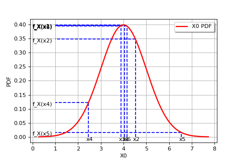
The following figure graphically illustrates the maximum likelihood method, in the particular case of a Gaussian probability distribution.
(Source code, png)
In general, in order to maximize the likelihood function classical optimization algorithms (e.g. gradient type) can be used. The Gaussian distribution case is an exception to this, as the maximum likelihood estimators are obtained analytically:
