Estimate a GEV on the Venice sea-levels data

In this example, we illustrate various techniques of extreme value modeling applied to the annual maximum sea-levels recorded in Venice over the period 1931-1981. Readers should refer to [coles2001] to get more details.

We illustrate techniques to:

• estimate a stationary GEV, using the -largest annual sea-levels for ,

using:

• the log-likelihood function,

• the profile log-likelihood function.

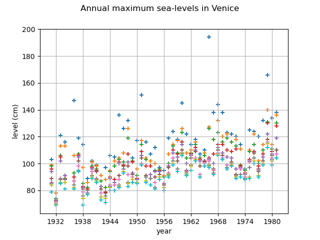
First, we load the 10 largest annual sea-levels in Venice. We start by looking at them through time. Note that for the year 1935, only the largest 6 observations are available. For simplicity of the example, we removed that year from the data but it could be used for all the analyses beased on the largest annual sea-levels for .

import openturns as ot
import openturns.viewer as otv
import openturns.experimental as otexp
from openturns.usecases import coles

data = coles.Coles().venice

The column contains the largest annual sea-levels.

print(data[:5])
graph = ot.Graph("Annual maximum sea-levels in Venice", "year", "level (cm)", True, "")
for r in range(10):
    cloud = ot.Cloud(data[:, [0, 1 + r]])
    graph.add(cloud)
graph.setIntegerXTick(True)
view = otv.View(graph)

    [ Year r1   r2   r3   r4   r5   r6   r7   r8   r9   r10  ]
0 : [ 1931  103   99   98   96   94   89   86   85   84   79 ]
1 : [ 1932   78   78   74   73   73   72   71   70   70   69 ]
2 : [ 1933  121  113  106  105  102   89   89   88   86   85 ]
3 : [ 1934  116  113   91   91   91   89   88   88   86   81 ]
4 : [ 1936  147  106   93   90   87   87   87   84   82   81 ]

Stationary GEV modeling from the annual maximum sea-levels

We first assume that the dependence through time is negligible, so we first model the data as independent observations over the observation period. We estimate the parameters of the GEV distribution by maximizing the log-likelihood of the data. We select the first column of the data.

sample = data[:, 1]

Estimate the parameters of the GEV by maximizing the log-likehood and compute the parameter distribution

factory = ot.GeneralizedExtremeValueFactory()
result_LL_max = factory.buildMethodOfLikelihoodMaximizationEstimator(sample)

We get the fitted GEV and its parameters of .

fitted_GEV = result_LL_max.getDistribution()
desc = fitted_GEV.getParameterDescription()
param = fitted_GEV.getParameter()
print(", ".join([f"{p}: {value:.3f}" for p, value in zip(desc, param)]))
print("Max log-likelihood (one max): ", result_LL_max.getLogLikelihood())

mu: 111.090, sigma: 17.340, xi: -0.077
Max log-likelihood (one max):  -218.85953988220427

We get the asymptotic distribution of the estimator . In that case, the asymptotic distribution is normal.

parameterEstimate = result_LL_max.getParameterDistribution()
print("Asymptotic distribution of the estimator : ")
print(parameterEstimate)

Asymptotic distribution of the estimator :
Normal(mu = [111.09,17.3401,-0.0770338], sigma = [2.90936,1.79642,0.0793379], R = [[  1         0.4502   -0.488149 ]
 [  0.4502    1        -0.438925 ]
 [ -0.488149 -0.438925  1        ]])

We get the covariance matrix and the standard deviation of .

print("Cov matrix = ", parameterEstimate.getCovariance())
print("Standard dev = ", parameterEstimate.getStandardDeviation())

Cov matrix =  [[  8.46436     2.35294    -0.112676   ]
 [  2.35294     3.22713    -0.0625576  ]
 [ -0.112676   -0.0625576   0.00629451 ]]
Standard dev =  [2.90936,1.79642,0.0793379]

We get the marginal confidence intervals of order 0.95.

order = 0.95
for i in range(3):
    ci = parameterEstimate.getMarginal(i).computeBilateralConfidenceInterval(order)
    print(desc[i] + ":", ci)

mu: [105.387, 116.792]
sigma: [13.8192, 20.861]
xi: [-0.232533, 0.0784657]

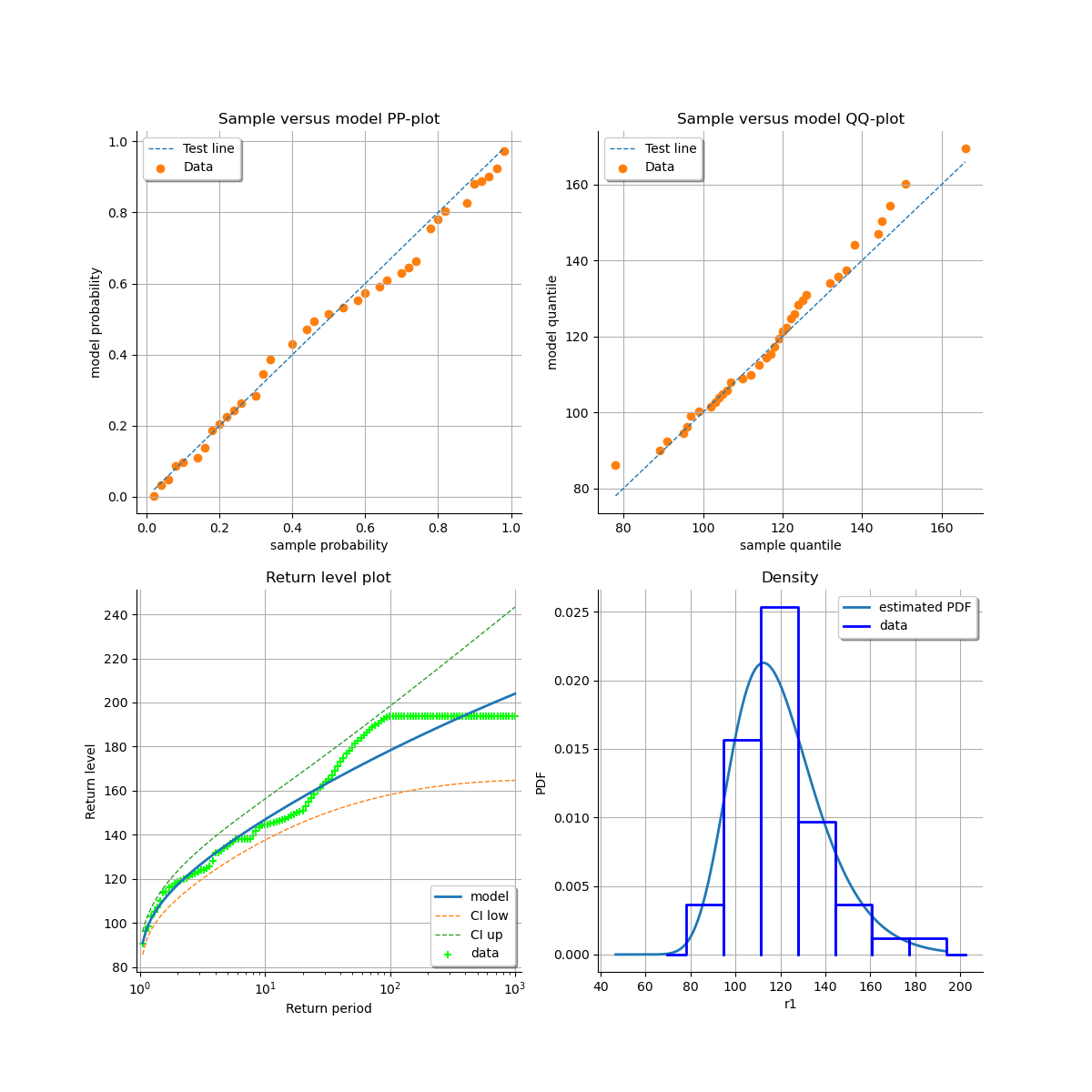
At last, we can validate the inference result thanks the 4 usual diagnostic plots:

• the probability-probability pot,

• the quantile-quantile pot,

• the return level plot,

• the empirical distribution function.

validation = otexp.GeneralizedExtremeValueValidation(result_LL_max, sample)
graph = validation.drawDiagnosticPlot()
view = otv.View(graph)

We can also use the profile log-likehood function rather than log-likehood function to estimate the parameters of the GEV.

result_PLL_max = factory.buildMethodOfProfileLikelihoodMaximizationEstimator(sample)

The following graph allows one to get the profile log-likelihood plot. It also indicates the optimal value of , the maximum profile log-likelihood and the confidence interval for of order 0.95 (which is the default value).

order = 0.95
result_PLL_max.setConfidenceLevel(order)
print(result_PLL_max.getParameterConfidenceInterval())

[-0.200118, 0.101776]

We can get the numerical values of the confidence interval: it appears to be a bit smaller with the interval obtained from the profile log-likelihood function than with the log-likelihood function. Note that if the order requested is too high, the confidence interval might not be calculated because one of its bound is out of the definition domain of the log-likelihood function.

try:
    print(
        "Confidence interval for xi = ", result_PLL_max.getParameterConfidenceInterval()
    )
except Exception as ex:
    print(type(ex))
    pass

Confidence interval for xi =  [-0.200118, 0.101776]

Stationary GEV modeling from the largest :math:`r` annual sea-levels

We still assume that the dependence through time is negligible. We estimate the parameters of the GEV distribution by maximizing the log-likelihood of the data. Now, we want to model more of the observed extremes than the annual maxima: the additional information contained in the largest observations can be used to improve the estimation of the GEV model.

Now, we drop the year column to keep only the maxima values.

sample_rmax = data[:, 1:]
print(sample_rmax[:5])

    [ r1  r2  r3  r4  r5  r6  r7  r8  r9  r10 ]
0 : [ 103  99  98  96  94  89  86  85  84  79 ]
1 : [  78  78  74  73  73  72  71  70  70  69 ]
2 : [ 121 113 106 105 102  89  89  88  86  85 ]
3 : [ 116 113  91  91  91  89  88  88  86  81 ]
4 : [ 147 106  93  90  87  87  87  84  82  81 ]

We estimate the parameters from the largest annual sea-levels for . For each value, we get the estimated parameters.

factory = ot.GeneralizedExtremeValueFactory()
r_candidate = [1, 5, 10]
for r in r_candidate:
    estimate = factory.buildMethodOfLikelihoodMaximization(sample_rmax, r)
    desc = estimate.getParameterDescription()
    p = estimate.getParameter()
    pretty_p = ", ".join([f"{param}: {value:.3f}" for param, value in zip(desc, p)])
    print(f"r={r:2} {pretty_p}")

r= 1 mu: 111.090, sigma: 17.340, xi: -0.077
r= 5 mu: 117.849, sigma: 13.423, xi: -0.087
r=10 mu: 116.868, sigma: 11.854, xi: -0.108

otv.View.ShowAll()