Note
Go to the end to download the full example code
Estimate tail dependence coefficients on the wind data
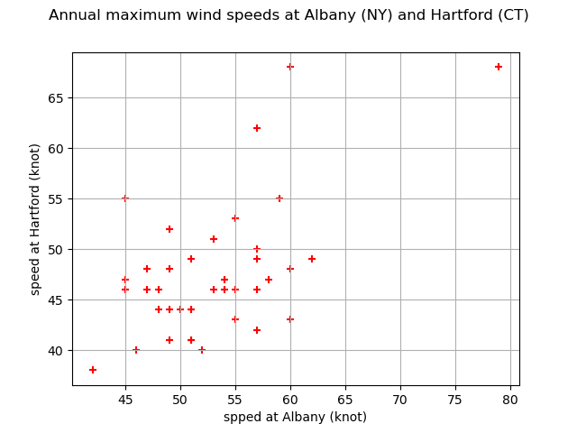
In this example we estimate the tail dependence coefficient of a bivariate sample applied to the corresponding annual maximum wind speeds over the period 1944-1983 at two locations in the United States: Albany, New-York and Hartford, Connecticut. Readers should refer to [coles2001] to get more details.
First, we load the wave_surge dataset. The speeds are expressed in knot : one knot is equalt to one nautical mile per hour, which means .
import openturns as ot
import openturns.viewer as otv
from openturns.usecases import coles

data = coles.Coles().wind[:, 1:]
print(data[:5])

graph = ot.Graph(
    "Annual maximum wind speeds at Albany (NY) and Hartford (CT)",
    "spped at Albany (knot)",
    "speed at Hartford (knot)",
    True,
    "",
)
cloud = ot.Cloud(data)
cloud.setColor("red")
graph.add(cloud)
view = otv.View(graph)

    [ Hartford Albany   ]
0 : [ 49       52       ]
1 : [ 54       46       ]
2 : [ 60       48       ]
3 : [ 49       44       ]
4 : [ 57       42       ]
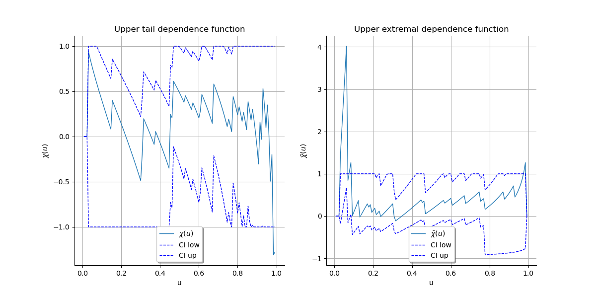
We plot the graph of the function and the graph of the function
. We conclude that both variables are asymptotially dependent
as
and that they are positively correlated as
.
We cn visually deduce the upper tail dependence coefficient
and
the upper extremal dependence coefficient
.
Note that the number of data points is so small that the curves seem chaotic.
It is difficult, if not impossible, to deduce the value of
and
from the curves.
graph1 = ot.VisualTest.DrawUpperTailDependenceFunction(data)
graph2 = ot.VisualTest.DrawUpperExtremalDependenceFunction(data)
grid = ot.GridLayout(1, 2)
grid.setGraph(0, 0, graph1)
grid.setGraph(0, 1, graph2)
view = otv.View(grid)

otv.View.ShowAll()
 OpenTURNS