Compute confidence intervals of a univariate noisy function

Introduction

In this example, we compute the pointwise confidence interval of the estimator of the conditional expectation given an input. We consider noisy observations of the sine function. Then we perform linear least squares regression to fit an order 4 polynomial. For a given point x, the code computes the confidence interval of the prediction y. This is the confidence interval of the conditional expectation given the input. Secondly, we compute the confidence interval of the noisy output observations. In this advanced example, we use the QRMethod low level class. Another example of this method is presented in Compute confidence intervals of a regression model from data.

import openturns as ot
import openturns.viewer as otv
import numpy as np


palette = ot.Drawable.BuildTableauPalette(5)

ot.RandomGenerator.SetSeed(0)

Compute the data

We generate noisy observations from the sine function. We define the function that we are going to approximate.

g = ot.SymbolicFunction(["x"], ["sin(2 * pi_ * x)"])

We plot the function depending on the input.

def plotFunction(g, color, lineStyle="dotted"):
    curve = g.draw(0.0, 1.0).getDrawable(0)
    curve.setColor(color)
    curve.setLineStyle("dotted")
    curve.setLegend("True")
    return curve


graph = ot.Graph("Polynomial curve fitting", "x", "y", True, "upper right")
# The "unknown" function
graph.add(plotFunction(g, palette[0]))
view = otv.View(graph)

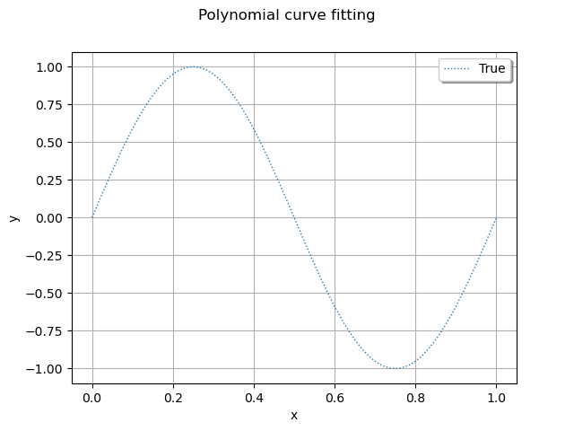
This is a nice, smooth function to approximate with polynomials.

def linearSample(xmin, xmax, npoints):
    """Returns a sample created from a regular grid
    from xmin to xmax with npoints points."""
    step = (xmax - xmin) / (npoints - 1)
    rg = ot.RegularGrid(xmin, step, npoints)
    vertices = rg.getVertices()
    return vertices

We consider observation points in the interval [0,1].

nTrain = 100
xTrain = linearSample(0, 1, nTrain)

Assume that the observations are noisy and that the noise follows a Normal distribution with zero mean and small standard deviation.

noise = ot.Normal(0, 0.5)
noiseSample = noise.getSample(nTrain)

The following code computes the observation as the sum of the function value and of the noise. The couple (xTrain,yTrain) is the training set: it is used to compute the coefficients of the polynomial model.

yTrain = g(xTrain) + noiseSample
print(yTrain[:5])

    [ y0         ]
0 : [  0.304101  ]
1 : [ -0.569663  ]
2 : [ -0.0925404 ]
3 : [  0.79199   ]
4 : [ -0.839545  ]

Then we plot the function and the observations.

def plotData(xTrain, yTrain, color, pointStyle="circle"):
    cloud = ot.Cloud(xTrain, yTrain)
    cloud.setPointStyle(pointStyle)
    cloud.setLegend("Observations")
    cloud.setColor(palette[1])
    return cloud


graph = ot.Graph("Polynomial curve fitting", "x", "y", True, "upper right")
# The "unknown" function
graph.add(plotFunction(g, palette[0]))
# Training set
graph.add(plotData(xTrain, yTrain, palette[1]))
view = otv.View(graph)

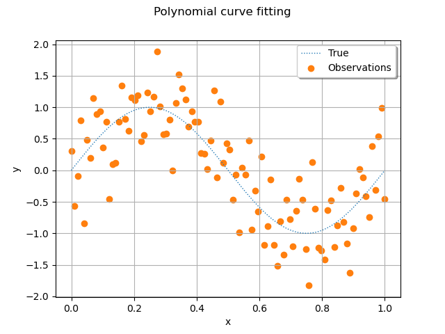
We see that the noisy observations of the function are relatively large compared to the function values. It may not be obvious that a regression model can fit that data well.

Compute the coefficients of the polynomial decomposition

In order to approximate the function with polynomials up to degree 4, we create a list of strings containing the associated monomials. We perform the loop from 0 up to totalDegree (but the range function takes totalDegree + 1 as its second input argument).

totalDegree = 4
polynomialCollection = [f"x^{degree}" for degree in range(0, totalDegree + 1)]
print(polynomialCollection)

['x^0', 'x^1', 'x^2', 'x^3', 'x^4']

Given the list of strings, we create a symbolic function which computes the values of the monomials.

basisFunction = ot.SymbolicFunction(["x"], polynomialCollection)
print(basisFunction)

[x]->[x^0,x^1,x^2,x^3,x^4]

Evaluate the design matrix as the value of the basis functions on the training sample.

designSampleTrain = basisFunction(xTrain)
print(designSampleTrain[:5])

    [ y0          y1          y2          y3          y4          ]
0 : [ 1           0           0           0           0           ]
1 : [ 1           0.010101    0.00010203  1.03061e-06 1.04102e-08 ]
2 : [ 1           0.020202    0.000408122 8.24488e-06 1.66563e-07 ]
3 : [ 1           0.030303    0.000918274 2.78265e-05 8.43226e-07 ]
4 : [ 1           0.040404    0.00163249  6.5959e-05  2.66501e-06 ]

Convert the design sample into a design matrix and create an instance of the QRMethod class. This class has the getGramInverse() method that we need to compute the confidence interval.

designMatrixTrain = ot.Matrix(designSampleTrain)
lsqMethod = ot.QRMethod(designMatrixTrain)

Solve the linear least squares problem and get the vector of coefficients.

betaHat = lsqMethod.solve(yTrain.asPoint())
print(betaHat)

[-0.193699,9.71586,-20.9196,-0.667074,12.5351]

Compute residuals and variance

We need to estimate the variance of the residuals. To do this we evaluate the predictions of the regression model on the training sample and compute the residuals.

yHatTrain = designMatrixTrain * betaHat
residuals = yHatTrain - yTrain.asPoint()
sampleSize = designMatrixTrain.getNbRows()
print("sampleSize=", sampleSize)
nParameters = designMatrixTrain.getNbColumns()
print("nParameters = ", nParameters)
sigma2Hat = residuals.normSquare() / (sampleSize - nParameters)
print("sigma2Hat = ", sigma2Hat)

sampleSize= 100
nParameters =  5
sigma2Hat =  0.25191909002749147

The couple (xTest,yHatTest) is the set where we want to evaluate the prediction confidence intervals. In order to evaluate the predictions from the regression model, multiply the design matrix evaluated on the test sample with the vector of coefficients.

nTest = 50
xTest = linearSample(0, 1, nTest)
designMatrixTest = ot.Matrix(basisFunction(xTest))
yHatTest = ot.Sample.BuildFromPoint(designMatrixTest * betaHat)

Then we plot the true function, its noisy observations and the least squares model of degree 4.

def plotPredictions(xTest, yHatTest, totalDegree, color):
    curve = ot.Curve(xTest, yHatTest)
    curve.setLegend(f"L.S. degree {totalDegree}")
    curve.setColor(color)
    return curve


graph = ot.Graph("Polynomial curve fitting", "x", "y", True, "upper right")
# The "unknown" function
graph.add(plotFunction(g, palette[0]))
# Training set
graph.add(plotData(xTrain, yTrain, palette[1]))
# Predictions
graph.add(plotPredictions(xTest, yHatTest, totalDegree, palette[2]))
view = otv.View(graph)

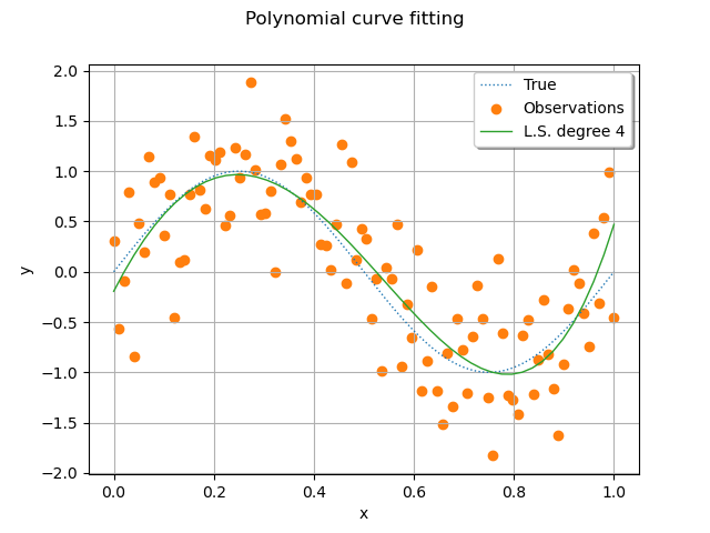
We see that the least squares polynomial model is relatively close to the true function.

Compute confidence intervals

The next function will help to compute confidence intervals. It is based on regression analysis.

def computeRegressionConfidenceInterval(
    lsqMethod,
    betaHat,
    sigma2Hat,
    designSample,
    alpha=0.95,
    mean=True,
    epsilonSigma=1.0e-5,
):
    """
    Compute a confidence interval for the estimate of the mean.

    Evaluates this confidence interval at points in the design matrix.

    This code is based on (Rawlings, Pantula & David, 1998)
    eq. 3.51 and 3.52 page 90.

    Parameters
    ----------
    lsqMethod: ot.LeastSquaresMethod
        The linear least squares method (e.g. QR or Cholesky).
    betaHat : ot.Point(parameterDimension)
        The solution of the least squares problem.
    sigma2Hat : float > 0.0
        The estimate of the variance.
    designSample : ot.Sample(size, parameterDimension)
        The design matrix of the linear model.
        This is the value of the functional basis depending on the
        input sample.
        Each row represents the input where the confidence interval
        is to be computed.
    alpha : float, in [0, 1]
        The width of the confidence interval.
    mean : bool
        If True, then computes the confidence interval of the mean.
        This interval contains yTrue = E[y|x] with probability alpha.
        Otherwise, computes a confidence interval of the prediction at point x.
        This interval contains y|x with probability alpha.
    epsilonSigma : float > 0.0
        A relatively small number. The minimal value of variance, which
        avoids a singular Normal distribution.

    Reference
    ---------
    - O. Rawlings John, G. Pantula Sastry, and A. Dickey David.
      Applied regression analysis—a research tool. Springer New York, 1998.

    Returns
    -------
    confidenceBounds : ot.Sample(size, 2)
        The first column contains the lower bound.
        The second column contains the upper bound.
    """

    inverseGram = lsqMethod.getGramInverse()
    sampleSize = designSample.getSize()
    confidenceBounds = ot.Sample(sampleSize, 2)
    for i in range(sampleSize):
        x0 = designSample[i, :]
        meanYHat = x0.dot(betaHat)
        sigma2YHat = x0.dot(inverseGram * x0) * sigma2Hat
        if not mean:
            sigma2YHat += sigma2Hat
        sigmaYHat = np.sqrt(sigma2YHat)
        sigmaYHat = max(epsilonSigma, sigmaYHat)  # Prevents a zero s.e.
        distribution = ot.Normal(meanYHat, sigmaYHat)
        interval = distribution.computeBilateralConfidenceInterval(alpha)
        lower = interval.getLowerBound()
        upper = interval.getUpperBound()
        confidenceBounds[i, 0] = lower[0]
        confidenceBounds[i, 1] = upper[0]
    return confidenceBounds

We evaluate the value of the basis functions on the test sample. This sample is used to compute the confidence interval.

designSampleTest = basisFunction(xTest)

Compute the confidence interval.

alpha = 0.95
confidenceIntervalMean = computeRegressionConfidenceInterval(
    lsqMethod, betaHat, sigma2Hat, designSampleTest, alpha=alpha
)

On output, the confidenceIntervalMean variable is a Sample of size 50 and dimension 2.

print(confidenceIntervalMean.getSize())

50

Plot the confidence interval (C.I.) of the pointwise estimator of the conditional expectation.

def plotConfidenceInterval(
    xTest, confidenceIntervalSample, color, lineStyle="dashed", label=""
):
    graph = ot.Graph()
    curve = ot.Curve(xTest, confidenceIntervalSample[:, 0])
    curve.setLegend(label)
    curve.setColor(color)
    curve.setLineStyle(lineStyle)
    graph.add(curve)
    curve = ot.Curve(xTest, confidenceIntervalSample[:, 1])
    curve.setLegend("")
    curve.setColor(color)
    curve.setLineStyle(lineStyle)
    graph.add(curve)
    return graph


graph = ot.Graph("Polynomial curve fitting", "x", "y", True, "upper right")
# The "unknown" function
graph.add(plotFunction(g, palette[0]))
# Training set
graph.add(plotData(xTrain, yTrain, palette[1]))
# Predictions
graph.add(plotPredictions(xTest, yHatTest, totalDegree, palette[2]))
# Confidence interval of the mean
graph.add(
    plotConfidenceInterval(
        xTest,
        confidenceIntervalMean,
        palette[3],
        label="Mean %.0f%%" % (100.0 * alpha),
    )
)
view = otv.View(graph)

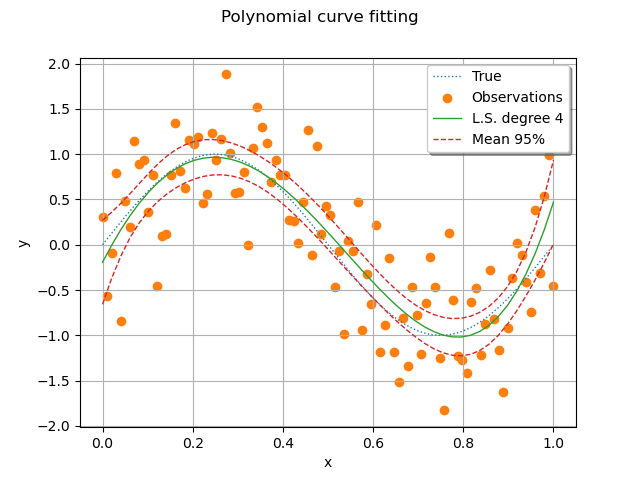
We see that the pointwise confidence interval contains the true model for most points. For a small set of points, there are points which are not within the bounds, but are not too far away. The observations, however, are not contained within these bounds. This is the goal of the next cell.

Finally, compute a 95% C.I. of the observations.

alpha = 0.95
confidenceIntervalObservations = computeRegressionConfidenceInterval(
    lsqMethod,
    betaHat,
    sigma2Hat,
    designSampleTest,
    alpha=alpha,
    mean=False,
)

Then we plot the function, its least squares approximation, the C.I. of the mean and the C.I. of the observations.

# sphinx_gallery_thumbnail_number = 5
graph = ot.Graph("Polynomial curve fitting", "x", "y", True, "upper right")
# The "unknown" function
graph.add(plotFunction(g, palette[0]))
# Training set
graph.add(plotData(xTrain, yTrain, palette[1]))
# Predictions
graph.add(plotPredictions(xTest, yHatTest, totalDegree, palette[2]))
# Confidence interval of the mean
graph.add(
    plotConfidenceInterval(
        xTest,
        confidenceIntervalMean,
        palette[3],
        label="Mean %.0f%%" % (100.0 * alpha),
    )
)
# Confidence interval of the observations.
graph.add(
    plotConfidenceInterval(
        xTest,
        confidenceIntervalObservations,
        palette[4],
        label="Obs. %.0f%%" % (100.0 * alpha),
    )
)
view = otv.View(graph)

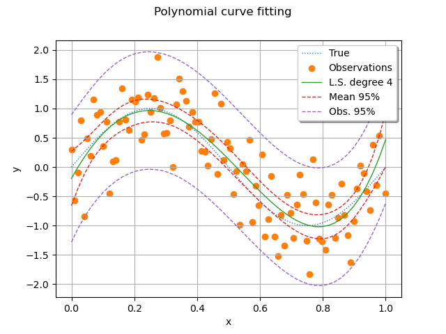
We see that the confidence interval of the observations contain most of the observations. The confidence interval of the observations is much larger than the C.I. of the mean, as expected from the statistical model.