Note
Go to the end to download the full example code
Create your own distribution given its quantile function
We want to create a distribution with CDF from the quantile function
.
In order to implement this, we use the
CompositeDistribution class.
We know that the random variable is distributed according to
if and only if
is distributed according to the uniform
distribution in the
interval, i.e.
.
Hence, if
then
is distributed according to
.
In this example, we want to create a distribution with CDF rho > 1`:
The quantile function is and writes:
Since , then
.
This is why we can simplify the expression and define the function
such as:
Then is distributed according to the
distribution.
First, we import the useful libraries and we create the symbolic function .
import openturns as ot
from openturns.viewer import View
Then, we create the function with
.
To do this, we create a function which takes both
and
as inputs and returns
.
Then the g function is defined as a
ParametricFunction with a fixed value of .
gWithParameter = ot.SymbolicFunction(["u", "rho"], ["log(-log(u)) / log(rho)"])
rho = 2.0
g = ot.ParametricFunction(gWithParameter, [1], [rho])
We define the distribution distF as the image through of the Uniform(0,1) distribution:
distF = ot.CompositeDistribution(g, ot.Uniform(0.0, 1.0))
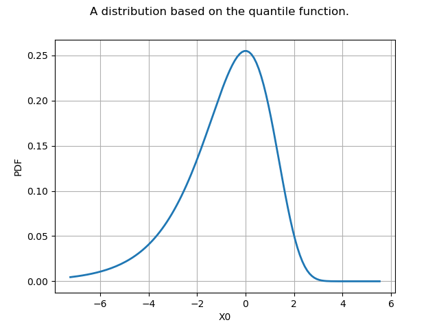
Now, we can draw its pdf, cdf, sample it,…
g = distF.drawPDF()
g.setTitle("A distribution based on the quantile function.")
g.setLegendPosition("")
view = View(g)
view.ShowAll()

 OpenTURNS