Note
Go to the end to download the full example code
Time variant system reliability problem
The objective is to evaluate the outcrossing rate from a safe to a failure domain in a time variant reliability problem.
We consider the following limit state function, defined as the difference between a degrading resistance and a time-varying load
:
The failure domaine is defined by:
which means that the resistance at is less than the stress at
.
We propose the following probabilistic model:
is the initial resistance, and
;
is the deterioration rate of the resistance; it is deterministic;
is the time-varying stress, which is modeled by a stationary Gaussian process of mean value
, standard deviation
and a squared exponential covariance model
.
The outcrossing rate from the safe to the failure domain at instant is defined by:
For each , we note the random variable
where
.
To evaluate , we need to consider the bivariate random vector
.
The event writes as the intersection of both events :
and
.
The objective is to evaluate:
1. Define some useful functions
We define the bivariate random vector .
Here,
is a bivariate Normal random vector:
with mean
and
with covariance matrix
defined by:
This function buils .
from math import sqrt
from openturns.viewer import View
import openturns as ot


def buildNormal(b, t, mu_S, covariance, delta_t=1e-5):
    sigma = ot.CovarianceMatrix(2)
    sigma[0, 0] = covariance(t, t)[0, 0]
    sigma[0, 1] = covariance(t, t + delta_t)[0, 0]
    sigma[1, 1] = covariance(t + delta_t, t + delta_t)[0, 0]
    return ot.Normal([b * t + mu_S, b * (t + delta_t) + mu_S], sigma)
This function creates the trivariate random vector where
is independent from
.
We need to create this random vector because both events
and
must be defined from the same random vector!
def buildCrossing(b, t, mu_S, covariance, R, delta_t=1e-5):
    normal = buildNormal(b, t, mu_S, covariance, delta_t)
    return ot.BlockIndependentDistribution([R, normal])
This function evaluates the probability using the Monte Carlo sampling. It defines the intersection event .
def getXEvent(b, t, mu_S, covariance, R, delta_t):
    full = buildCrossing(b, t, mu_S, covariance, R, delta_t)
    X = ot.RandomVector(full)
    f1 = ot.SymbolicFunction(["R", "X1", "X2"], ["X1 - R"])
    e1 = ot.ThresholdEvent(ot.CompositeRandomVector(f1, X), ot.Less(), 0.0)
    f2 = ot.SymbolicFunction(["R", "X1", "X2"], ["X2 - R"])
    e2 = ot.ThresholdEvent(ot.CompositeRandomVector(f2, X), ot.GreaterOrEqual(), 0.0)
    event = ot.IntersectionEvent([e1, e2])
    return X, event
def computeCrossingProbability_MonteCarlo(
    b, t, mu_S, covariance, R, delta_t, n_block, n_iter, CoV
):
    X, event = getXEvent(b, t, mu_S, covariance, R, delta_t)
    algo = ot.ProbabilitySimulationAlgorithm(event, ot.MonteCarloExperiment())
    algo.setBlockSize(n_block)
    algo.setMaximumOuterSampling(n_iter)
    algo.setMaximumCoefficientOfVariation(CoV)
    algo.run()
    return algo.getResult().getProbabilityEstimate() / delta_t
This function evaluates the probability using the Low Discrepancy sampling.
def computeCrossingProbability_QMC(
    b, t, mu_S, covariance, R, delta_t, n_block, n_iter, CoV
):
    X, event = getXEvent(b, t, mu_S, covariance, R, delta_t)
    algo = ot.ProbabilitySimulationAlgorithm(
        event,
        ot.LowDiscrepancyExperiment(ot.SobolSequence(X.getDimension()), n_block, False),
    )
    algo.setBlockSize(n_block)
    algo.setMaximumOuterSampling(n_iter)
    algo.setMaximumCoefficientOfVariation(CoV)
    algo.run()
    return algo.getResult().getProbabilityEstimate() / delta_t
This function evaluates the probability using the FORM algorithm for event systems..
def computeCrossingProbability_FORM(b, t, mu_S, covariance, R, delta_t):
    X, event = getXEvent(b, t, mu_S, covariance, R, delta_t)
    algo = ot.SystemFORM(ot.SQP(), event, X.getMean())
    algo.run()
    return algo.getResult().getEventProbability() / delta_t
2. Evaluate the probability
First, fix some parameters: and the covariance model which is the Squared Exponential model.
Be careful to the parameter
which is of great importance: if it is too small, the simulation methods have problems to converge
because the correlation rate is too high between the instants
and
.
We advice to take
.
mu_S = 3.0
sigma_S = 0.5
ll = 10

b = 0.01

mu_R = 5.0
sigma_R = 0.3
R = ot.Normal(mu_R, sigma_R)

covariance = ot.SquaredExponential([ll / sqrt(2)], [sigma_S])

t0 = 0.0
t1 = 50.0
N = 26

# Get all the time steps t
times = ot.RegularGrid(t0, (t1 - t0) / (N - 1.0), N).getVertices()

delta_t = 1e-1
Use all the methods previously described:
Monte Carlo: values in values_MC
Low discrepancy suites: values in values_QMC
FORM: values in values_FORM
values_MC = list()
values_QMC = list()
values_FORM = list()

for tick in times:
    values_MC.append(
        computeCrossingProbability_MonteCarlo(
            b, tick[0], mu_S, covariance, R, delta_t, 2**12, 2**3, 1e-2
        )
    )
    values_QMC.append(
        computeCrossingProbability_QMC(
            b, tick[0], mu_S, covariance, R, delta_t, 2**12, 2**3, 1e-2
        )
    )
    values_FORM.append(
        computeCrossingProbability_FORM(b, tick[0], mu_S, covariance, R, delta_t)
    )
print("Values MC = ", values_MC)
print("Values QMC = ", values_QMC)
print("Values FORM = ", values_FORM)
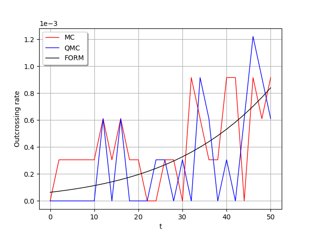
Values MC =  [0.0, 0.00030517578125, 0.00030517578125, 0.00030517578125, 0.00030517578125, 0.00030517578125, 0.0006103515625, 0.00030517578125, 0.0006103515625, 0.00030517578125, 0.00030517578125, 0.0, 0.0, 0.00030517578125, 0.00030517578125, 0.0, 0.00091552734375, 0.0006103515625, 0.00030517578125, 0.00030517578125, 0.00091552734375, 0.00091552734375, 0.0, 0.00091552734375, 0.0006103515625, 0.00091552734375]
Values QMC =  [0.0, 0.0, 0.0, 0.0, 0.0, 0.0, 0.0006103515625, 0.0, 0.0006103515625, 0.0, 0.0, 0.0, 0.00030517578125, 0.00030517578125, 0.0, 0.00030517578125, 0.0, 0.00091552734375, 0.0006103515625, 0.0, 0.00030517578125, 0.0, 0.0006103515625, 0.001220703125, 0.00091552734375, 0.0006103515625]
Values FORM =  [6.407247221976507e-05, 7.202731340749856e-05, 8.087457586090277e-05, 9.070184981054664e-05, 0.00010160352566970394, 0.00011368175073412876, 0.0001270463113912958, 0.00014181491000870818, 0.00015811435561607578, 0.00017607979215241996, 0.00019585595886454746, 0.0002175971126689752, 0.0002414674407523497, 0.0002676410518535999, 0.0002963031343688264, 0.0003276489835870634, 0.00036188514225255717, 0.00039922842206094566, 0.0004399070455775222, 0.000484160922259269, 0.0005322401306923784, 0.0005844062178174964, 0.0006409303353549688, 0.000702094564935671, 0.0007681919118323028, 0.0008395236033398269]
Draw the graphs!
g = ot.Graph()
g.setAxes(True)
g.setGrid(True)
c = ot.Curve(times, [[p] for p in values_MC])
g.add(c)
c = ot.Curve(times, [[p] for p in values_QMC])
g.add(c)
c = ot.Curve(times, [[p] for p in values_FORM])
g.add(c)
g.setLegends(["MC", "QMC", "FORM"])
g.setColors(["red", "blue", "black"])
g.setLegendPosition("upper left")
g.setXTitle("t")
g.setYTitle("Outcrossing rate")
view = View(g)
view.ShowAll()

Total running time of the script: (0 minutes 2.148 seconds)
 OpenTURNS