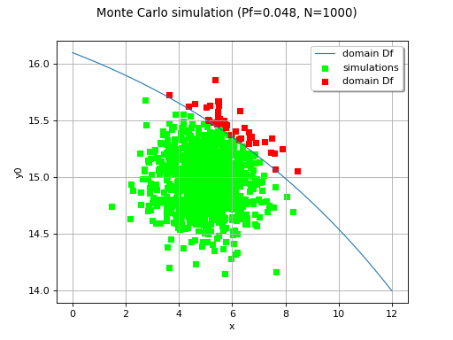
Monte Carlo simulation
Using the probability distribution the probability distribution of a random
vector  , we seek to evaluate the following probability:

Here, is a random vector,  a deterministic
vector,
a deterministic
vector,  the function known as limit state function
which enables the definition of the event
the function known as limit state function
which enables the definition of the event  .
.
If we have the set  of N
independent samples of the random vector ,
we can estimate
of N
independent samples of the random vector ,
we can estimate  as follows:

where  describes the indicator function equal to 1 if
  and equal to 0 otherwise; the idea here is in fact to estimate the required
probability by the proportion of cases, among the N samples of ,
for which the event
and equal to 0 otherwise; the idea here is in fact to estimate the required
probability by the proportion of cases, among the N samples of ,
for which the event  occurs.
By the law of large numbers, we know that this estimation converges to the
required value  as the sample size N tends to infinity.
The Central Limit Theorem allows one to build an asymptotic confidence interval using the normal limit distribution as follows:
![\lim_{N\rightarrow\infty}\Prob{P_f\in[\widehat{P}_{f,\inf},\widehat{P}_{f,\sup}]} = \alpha](data:image/svg+xml;base64,PD94bWwgdmVyc2lvbj0nMS4wJyBlbmNvZGluZz0nVVRGLTgnPz4KPCEtLSBUaGlzIGZpbGUgd2FzIGdlbmVyYXRlZCBieSBkdmlzdmdtIDMuMiAtLT4KPHN2ZyB2ZXJzaW9uPScxLjEnIHhtbG5zPSdodHRwOi8vd3d3LnczLm9yZy8yMDAwL3N2ZycgeG1sbnM6eGxpbms9J2h0dHA6Ly93d3cudzMub3JnLzE5OTkveGxpbmsnIHdpZHRoPScxNjUuNDYzMDM2cHQnIGhlaWdodD0nMjEuNTE5NTIycHQnIHZpZXdCb3g9JzExMS41Mzk5NjIgLTIyLjM4MjgyMyAxNjUuNDYzMDM2IDIxLjUxOTUyMic+CjxkZWZzPgo8cGF0aCBpZD0nZzYtMTAyJyBkPSdNMS41MjIyOTEtMy4xNzIxMDVIMi40Nzg3MDVWLTMuNDM1MTE4SDEuNDk4MzgxVi00LjMzNTc0MUMxLjQ5ODM4MS01LjAyOTE0MSAxLjg4ODkxNy01LjM4Nzc5NiAyLjIzOTYwMS01LjM4Nzc5NkMyLjM2NzEyMy01LjM4Nzc5NiAyLjQzODg1NC01LjM1NTkxNSAyLjQ3MDczNS01LjM0Nzk0NUMyLjMyNzI3My01LjI3NjIxNCAyLjI4NzQyMi01LjE0MDcyMiAyLjI4NzQyMi01LjAzNzExMUMyLjI4NzQyMi00LjgyOTg4OCAyLjQzODg1NC00LjY3ODQ1NiAyLjY0NjA3Ny00LjY3ODQ1NkMyLjg2MTI3LTQuNjc4NDU2IDMuMDA0NzMyLTQuODI5ODg4IDMuMDA0NzMyLTUuMDM3MTExQzMuMDA0NzMyLTUuMzc5ODI2IDIuNjY5OTg4LTUuNjEwOTU5IDIuMjQ3NTcyLTUuNjEwOTU5QzEuNjQ5ODEzLTUuNjEwOTU5IC45NDA0NzMtNS4xODA1NzMgLjk0MDQ3My00LjMyNzc3MVYtMy40MzUxMThILjI4NjkyNFYtMy4xNzIxMDVILjk0MDQ3M1YtLjYyMTY2OUMuOTQwNDczLS4yNjMwMTQgLjg0NDgzMi0uMjYzMDE0IC4zMzQ3NDUtLjI2MzAxNFYwQy42NDU1NzktLjAyMzkxIDEuMDgzOTM1LS4wMjM5MSAxLjI3NTIxOC0uMDIzOTFDMS43NDU0NTUtLjAyMzkxIDEuNzYxMzk1LS4wMjM5MSAyLjI3OTQ1MiAwVi0uMjYzMDE0SDIuMTIwMDVDMS41MzgyMzItLjI2MzAxNCAxLjUyMjI5MS0uMzUwNjg1IDEuNTIyMjkxLS42Mzc2MDlWLTMuMTcyMTA1WicvPgo8cGF0aCBpZD0nZzYtMTA1JyBkPSdNMS41NTQxNzItNC45MDk1ODlDMS41NTQxNzItNS4xNDA3MjIgMS4zNzA4NTktNS4zNTU5MTUgMS4xMDc4NDYtNS4zNTU5MTVDLjg3NjcxMi01LjM1NTkxNSAuNjY5NDg5LTUuMTcyNjAzIC42Njk0ODktNC45MTc1NTlDLjY2OTQ4OS00LjYzODYwNSAuOTAwNjIzLTQuNDcxMjMzIDEuMTA3ODQ2LTQuNDcxMjMzQzEuMzg2OC00LjQ3MTIzMyAxLjU1NDE3Mi00LjcwMjM2NiAxLjU1NDE3Mi00LjkwOTU4OVpNLjM1ODY1NS0zLjQyNzE0OFYtMy4xNjQxMzRDLjg2ODc0Mi0zLjE2NDEzNCAuOTQwNDczLTMuMTE2MzE0IC45NDA0NzMtMi43MjU3NzhWLS42MjE2NjlDLjk0MDQ3My0uMjYzMDE0IC44NDQ4MzItLjI2MzAxNCAuMzM0NzQ1LS4yNjMwMTRWMEMuNjQ1NTc5LS4wMjM5MSAxLjA5MTkwNS0uMDIzOTEgMS4yMTE0NTctLjAyMzkxQzEuMzE1MDY4LS4wMjM5MSAxLjc5MzI3NS0uMDIzOTEgMi4wNzIyMjkgMFYtLjI2MzAxNEMxLjU1NDE3Mi0uMjYzMDE0IDEuNTIyMjkxLS4zMDI4NjQgMS41MjIyOTEtLjYxMzY5OVYtMy41MTQ4MTlMLjM1ODY1NS0zLjQyNzE0OFonLz4KPHBhdGggaWQ9J2c2LTExMCcgZD0nTTMuODczNDc0LTIuNDE0OTQ0QzMuODczNDc0LTMuMDg0NDMzIDMuNTcwNjEtMy41MTQ4MTkgMi43MzM3NDgtMy41MTQ4MTlDMS45NDQ3MDctMy41MTQ4MTkgMS41ODYwNTItMi45NDA5NzEgMS40OTA0MTEtMi43NDk2ODlIMS40ODI0NDFWLTMuNTE0ODE5TC4zMjY3NzUtMy40MjcxNDhWLTMuMTY0MTM0Qy44Njg3NDItMy4xNjQxMzQgLjkzMjUwMy0zLjEwODM0NCAuOTMyNTAzLTIuNzE3ODA4Vi0uNjIxNjY5Qy45MzI1MDMtLjI2MzAxNCAuODM2ODYyLS4yNjMwMTQgLjMyNjc3NS0uMjYzMDE0VjBDLjY2OTQ4OS0uMDIzOTEgMS4wMjAxNzQtLjAyMzkxIDEuMjM1MzY3LS4wMjM5MUMxLjQ2NjUwMS0uMDIzOTEgMS44MDEyNDUtLjAyMzkxIDIuMTQzOTYgMFYtLjI2MzAxNEMxLjYzMzg3My0uMjYzMDE0IDEuNTM4MjMyLS4yNjMwMTQgMS41MzgyMzItLjYyMTY2OVYtMi4wNjQyNTlDMS41MzgyMzItMi45MDExMjEgMi4xNzU4NDEtMy4yOTE2NTYgMi42NjIwMTctMy4yOTE2NTZTMy4yNjc3NDYtMi45NDg5NDEgMy4yNjc3NDYtMi40NDY4MjRWLS42MjE2NjlDMy4yNjc3NDYtLjI2MzAxNCAzLjE3MjEwNS0uMjYzMDE0IDIuNjYyMDE3LS4yNjMwMTRWMEMzLjAwNDczMi0uMDIzOTEgMy4zNTU0MTctLjAyMzkxIDMuNTcwNjEtLjAyMzkxQzMuODAxNzQzLS4wMjM5MSA0LjEzNjQ4OC0uMDIzOTEgNC40NzkyMDMgMFYtLjI2MzAxNEMzLjk2OTExNi0uMjYzMDE0IDMuODczNDc0LS4yNjMwMTQgMy44NzM0NzQtLjYyMTY2OVYtMi40MTQ5NDRaJy8+CjxwYXRoIGlkPSdnNi0xMTInIGQ9J00yLjA5NjEzOSAxLjI4MzE4OEMxLjU4NjA1MiAxLjI4MzE4OCAxLjQ5MDQxMSAxLjI4MzE4OCAxLjQ5MDQxMSAuOTI0NTMzVi0uMzkwNTM1QzEuODY1MDA2IC4wMTU5NCAyLjI3MTQ4MiAuMDc5NzAxIDIuNTI2NTI2IC4wNzk3MDFDMy41Mzg3MyAuMDc5NzAxIDQuNDE1NDQyLS43MDEzNyA0LjQxNTQ0Mi0xLjcyMTU0NEM0LjQxNTQ0Mi0yLjcxNzgwOCAzLjYxMDQ2MS0zLjUxNDgxOSAyLjY0NjA3Ny0zLjUxNDgxOUMyLjMzNTI0My0zLjUxNDgxOSAxLjg3Mjk3Ni0zLjQzNTExOCAxLjQ2NjUwMS0zLjAyMDY3MlYtMy41MTQ4MTlMLjI3ODk1NC0zLjQyNzE0OFYtMy4xNjQxMzRDLjg0NDgzMi0zLjE2NDEzNCAuODg0NjgyLTMuMTE2MzE0IC44ODQ2ODItMi43ODE1NjlWLjkyNDUzM0MuODg0NjgyIDEuMjgzMTg4IC43ODkwNDEgMS4yODMxODggLjI3ODk1NCAxLjI4MzE4OFYxLjU0NjIwMkMuNjIxNjY5IDEuNTIyMjkxIC45NzIzNTQgMS41MjIyOTEgMS4xODc1NDcgMS41MjIyOTFDMS40MTg2OCAxLjUyMjI5MSAxLjc1MzQyNSAxLjUyMjI5MSAyLjA5NjEzOSAxLjU0NjIwMlYxLjI4MzE4OFpNMS40OTA0MTEtMi42NTQwNDdDMS42NzM3MjQtMi45NzI4NTIgMi4wNzIyMjktMy4yNjc3NDYgMi41NzQzNDYtMy4yNjc3NDZDMy4xODgwNDUtMy4yNjc3NDYgMy43MDYxMDItMi41OTAyODYgMy43MDYxMDItMS43MjE1NDRDMy43MDYxMDItLjgwNDk4MSAzLjEzMjI1NC0uMTQzNDYyIDIuNDg2Njc1LS4xNDM0NjJDMi4yMDc3MjEtLjE0MzQ2MiAxLjg0MTA5Ni0uMjYzMDE0IDEuNTg2MDUyLS42NjE1MTlDMS40OTA0MTEtLjc5NzAxMSAxLjQ5MDQxMS0uODA0OTgxIDEuNDkwNDExLS45NTY0MTNWLTIuNjU0MDQ3WicvPgo8cGF0aCBpZD0nZzYtMTE1JyBkPSdNMi44MzczNi0zLjM0NzQ0N0MyLjgzNzM2LTMuNDc0OTY5IDIuODM3MzYtMy41NTQ2NyAyLjczMzc0OC0zLjU1NDY3QzIuNjkzODk4LTMuNTU0NjcgMi42Njk5ODgtMy41NTQ2NyAyLjU0MjQ2Ni0zLjQyNzE0OEMyLjUyNjUyNi0zLjQxOTE3OCAyLjQ1NDc5NS0zLjM0NzQ0NyAyLjQzMDg4NC0zLjM0NzQ0N0MyLjQyMjkxNC0zLjM0NzQ0NyAyLjQwNjk3NC0zLjM0NzQ0NyAyLjM1OTE1My0zLjM3OTMyOEMyLjIzMTYzMS0zLjQ2Njk5OSAyLjAwMDQ5OC0zLjU1NDY3IDEuNjQxODQzLTMuNTU0NjdDLjUyNjAyNy0zLjU1NDY3IC4yNzg5NTQtMi45NDg5NDEgLjI3ODk1NC0yLjU2NjM3NkMuMjc4OTU0LTIuMTY3ODcgLjU3Mzg0OC0xLjkzNjczNyAuNTk3NzU4LTEuOTEyODI3Qy45MTY1NjMtMS42NzM3MjQgMS4wOTk4NzUtMS42NDE4NDMgMS42MzM4NzMtMS41NDYyMDJDMi4wMDg0NjgtMS40NzQ0NzEgMi42MjIxNjctMS4zNjI4ODkgMi42MjIxNjctLjgyMDkyMkMyLjYyMjE2Ny0uNTEwMDg3IDIuNDE0OTQ0LS4xNDM0NjIgMS42ODE2OTQtLjE0MzQ2MkMuODc2NzEyLS4xNDM0NjIgLjY0NTU3OS0uNzY1MTMxIC41NDE5NjgtMS4xODc1NDdDLjUxMDA4Ny0xLjI5MTE1OCAuNTAyMTE3LTEuMzMxMDA5IC40MDY0NzYtMS4zMzEwMDlDLjI3ODk1NC0xLjMzMTAwOSAuMjc4OTU0LTEuMjY3MjQ4IC4yNzg5NTQtMS4xMTU4MTZWLS4xMjc1MjJDLjI3ODk1NCAwIC4yNzg5NTQgLjA3OTcwMSAuMzgyNTY1IC4wNzk3MDFDLjQzMDM4NiAuMDc5NzAxIC40MzgzNTYgLjA3MTczMSAuNTgxODE4LS4wNzk3MDFDLjYyMTY2OS0uMTE5NTUyIC43MDkzNC0uMjIzMTYzIC43NDkxOTEtLjI2MzAxNEMxLjEwNzg0NiAuMDYzNzYxIDEuNDgyNDQxIC4wNzk3MDEgMS42ODk2NjQgLjA3OTcwMUMyLjcwMTg2OCAuMDc5NzAxIDMuMDUyNTUzLS41MDIxMTcgMy4wNTI1NTMtMS4wMjgxNDRDMy4wNTI1NTMtMS40MTA3MSAyLjgyMTQyLTEuOTY4NjE4IDEuODcyOTc2LTIuMTQzOTZDMS44MDkyMTUtMi4xNTk5IDEuMzYyODg5LTIuMjM5NjAxIDEuMzMxMDA5LTIuMjM5NjAxQzEuMDgzOTM1LTIuMjk1MzkyIC43MDkzNC0yLjQ2Mjc2NSAuNzA5MzQtMi43ODE1NjlDLjcwOTM0LTMuMDIwNjcyIC44ODQ2ODItMy4zNTU0MTcgMS42NDE4NDMtMy4zNTU0MTdDMi41MzQ0OTYtMy4zNTU0MTcgMi41NzQzNDYtMi43MDE4NjggMi41OTAyODYtMi40Nzg3MDVDMi41OTgyNTctMi40MTQ5NDQgMi42NTQwNDctMi4zOTEwMzQgMi43MDk4MzgtMi4zOTEwMzRDMi44MzczNi0yLjM5MTAzNCAyLjgzNzM2LTIuNDQ2ODI0IDIuODM3MzYtMi41OTgyNTdWLTMuMzQ3NDQ3WicvPgo8cGF0aCBpZD0nZzYtMTE3JyBkPSdNMi42NjIwMTctMy40MjcxNDhWLTMuMTY0MTM0QzMuMjAzOTg1LTMuMTY0MTM0IDMuMjY3NzQ2LTMuMTA4MzQ0IDMuMjY3NzQ2LTIuNzE3ODA4Vi0xLjMzMTAwOUMzLjI2Nzc0Ni0uNjQ1NTc5IDIuODUzMy0uMTQzNDYyIDIuMjU1NTQyLS4xNDM0NjJDMS41NzAxMTItLjE0MzQ2MiAxLjUzODIzMi0uNDg2MTc3IDEuNTM4MjMyLS44ODQ2ODJWLTMuNTE0ODE5TC4zMjY3NzUtMy40MjcxNDhWLTMuMTY0MTM0Qy45MzI1MDMtMy4xNjQxMzQgLjkzMjUwMy0zLjE0MDIyNCAuOTMyNTAzLTIuNDMwODg0Vi0xLjIzNTM2N0MuOTMyNTAzLS42NjE1MTkgLjkzMjUwMyAuMDc5NzAxIDIuMjA3NzIxIC4wNzk3MDFDMi45NTY5MTIgLjA3OTcwMSAzLjI0MzgzNi0uNDk0MTQ3IDMuMjgzNjg2LS41NjU4NzhIMy4yOTE2NTZWLjA3OTcwMUw0LjQ3OTIwMyAwVi0uMjYzMDE0QzMuOTM3MjM1LS4yNjMwMTQgMy44NzM0NzQtLjMxODgwNCAzLjg3MzQ3NC0uNzA5MzRWLTMuNTE0ODE5TDIuNjYyMDE3LTMuNDI3MTQ4WicvPgo8cGF0aCBpZD0nZzUtMTEnIGQ9J001LjUzNTI0My0zLjAyNDY1OEM1LjUzNTI0My00LjE4NDMwOSA0Ljg3NzcwOS01LjI3MjIyOSAzLjYxMDQ2MS01LjI3MjIyOUMyLjA0NDMzNC01LjI3MjIyOSAuNDc4MjA3LTMuNTYyNjQgLjQ3ODIwNy0xLjg2NTAwNkMuNDc4MjA3LS44MjQ5MDcgMS4xMjM3ODYgLjExOTU1MiAyLjM0MzIxMyAuMTE5NTUyQzMuMDg0NDMzIC4xMTk1NTIgMy45NjkxMTYtLjE2NzM3MiA0LjgxNzkzMy0uODg0NjgyQzQuOTg1MzA1LS4yMTUxOTMgNS4zNTU5MTUgLjExOTU1MiA1Ljg2OTk4OCAuMTE5NTUyQzYuNTE1NTY3IC4xMTk1NTIgNi44MzgzNTYtLjU0OTkzOCA2LjgzODM1Ni0uNzA1MzU1QzYuODM4MzU2LS44MTI5NTEgNi43NTQ2Ny0uODEyOTUxIDYuNzE4ODA0LS44MTI5NTFDNi42MjMxNjMtLjgxMjk1MSA2LjYxMTIwOC0uNzc3MDg2IDYuNTc1MzQyLS42ODE0NDVDNi40Njc3NDYtLjM4MjU2NSA2LjE5Mjc3Ny0uMTE5NTUyIDUuOTA1ODUzLS4xMTk1NTJDNS41MzUyNDMtLjExOTU1MiA1LjUzNTI0My0uODg0NjgyIDUuNTM1MjQzLTEuNjEzOTQ4QzYuNzU0NjctMy4wNzI0NzggNy4wNDE1OTQtNC41Nzg4MjkgNy4wNDE1OTQtNC41OTA3ODVDNy4wNDE1OTQtNC42OTgzODEgNi45NDU5NTMtNC42OTgzODEgNi45MTAwODctNC42OTgzODFDNi44MDI0OTEtNC42OTgzODEgNi43OTA1MzUtNC42NjI1MTYgNi43NDI3MTUtNC40NDczMjNDNi41ODcyOTgtMy45MjEyOTUgNi4yNzY0NjMtMi45ODg3OTIgNS41MzUyNDMtMi4wMDg0NjhWLTMuMDI0NjU4Wk00Ljc4MjA2Ny0xLjE3MTYwNkMzLjczMDAxMi0uMjI3MTQ4IDIuNzg1NTU0LS4xMTk1NTIgMi4zNjcxMjMtLjExOTU1MkMxLjUxODMwNi0uMTE5NTUyIDEuMjc5MjAzLS44NzI3MjcgMS4yNzkyMDMtMS40MzQ2MkMxLjI3OTIwMy0xLjk0ODY5MiAxLjU0MjIxNy0zLjE2ODEyIDEuOTEyODI3LTMuODI1NjU0QzIuNDAyOTg5LTQuNjYyNTE2IDMuMDcyNDc4LTUuMDMzMTI2IDMuNjEwNDYxLTUuMDMzMTI2QzQuNzcwMTEyLTUuMDMzMTI2IDQuNzcwMTEyLTMuNTE0ODE5IDQuNzcwMTEyLTIuNTEwNTg1QzQuNzcwMTEyLTIuMjExNzA2IDQuNzU4MTU3LTEuOTAwODcyIDQuNzU4MTU3LTEuNjAxOTkzQzQuNzU4MTU3LTEuMzYyODg5IDQuNzcwMTEyLTEuMzAzMTEzIDQuNzgyMDY3LTEuMTcxNjA2WicvPgo8cGF0aCBpZD0nZzUtNTknIGQ9J00yLjMzMTI1OCAuMDQ3ODIxQzIuMzMxMjU4LS42NDU1NzkgMi4xMDQxMS0xLjE1OTY1MSAxLjYxMzk0OC0xLjE1OTY1MUMxLjIzMTM4Mi0xLjE1OTY1MSAxLjA0MDEtLjg0ODgxNyAxLjA0MDEtLjU4NTgwM1MxLjIxOTQyNyAwIDEuNjI1OTAzIDBDMS43ODEzMiAwIDEuOTEyODI3LS4wNDc4MjEgMi4wMjA0MjMtLjE1NTQxN0MyLjA0NDMzNC0uMTc5MzI4IDIuMDU2Mjg5LS4xNzkzMjggMi4wNjgyNDQtLjE3OTMyOEMyLjA5MjE1NC0uMTc5MzI4IDIuMDkyMTU0LS4wMTE5NTUgMi4wOTIxNTQgLjA0NzgyMUMyLjA5MjE1NCAuNDQyMzQxIDIuMDIwNDIzIDEuMjE5NDI3IDEuMzI3MDI0IDEuOTk2NTEzQzEuMTk1NTE3IDIuMTM5OTc1IDEuMTk1NTE3IDIuMTYzODg1IDEuMTk1NTE3IDIuMTg3Nzk2QzEuMTk1NTE3IDIuMjQ3NTcyIDEuMjU1MjkzIDIuMzA3MzQ3IDEuMzE1MDY4IDIuMzA3MzQ3QzEuNDEwNzEgMi4zMDczNDcgMi4zMzEyNTggMS40MjI2NjUgMi4zMzEyNTggLjA0NzgyMVonLz4KPHBhdGggaWQ9J2c1LTgwJyBkPSdNMy41Mzg3My0zLjgwMTc0M0g1LjU0NzE5OEM3LjE5NzAxMS0zLjgwMTc0MyA4Ljg0NjgyNC01LjAyMTE3MSA4Ljg0NjgyNC02LjM4NDA2QzguODQ2ODI0LTcuMzE2NTYzIDguMDU3NzgzLTguMTY1MzggNi41NTE0MzItOC4xNjUzOEgyLjg1NzI4NUMyLjYzMDEzNy04LjE2NTM4IDIuNTIyNTQtOC4xNjUzOCAyLjUyMjU0LTcuOTM4MjMyQzIuNTIyNTQtNy44MTg2OCAyLjYzMDEzNy03LjgxODY4IDIuODA5NDY1LTcuODE4NjhDMy41Mzg3My03LjgxODY4IDMuNTM4NzMtNy43MjMwMzkgMy41Mzg3My03LjU5MTUzMkMzLjUzODczLTcuNTY3NjIxIDMuNTM4NzMtNy40OTU4OSAzLjQ5MDkwOS03LjMxNjU2M0wxLjg3Njk2MS0uODg0NjgyQzEuNzY5MzY1LS40NjYyNTIgMS43NDU0NTUtLjM0NjcgLjkwODU5My0uMzQ2N0MuNjgxNDQ1LS4zNDY3IC41NjE4OTMtLjM0NjcgLjU2MTg5My0uMTMxNTA3Qy41NjE4OTMgMCAuNjY5NDg5IDAgLjc0MTIyIDBDLjk2ODM2OSAwIDEuMjA3NDcyLS4wMjM5MSAxLjQzNDYyLS4wMjM5MUgyLjgzMzM3NUMzLjA2MDUyMy0uMDIzOTEgMy4zMTE1ODIgMCAzLjUzODczIDBDMy42MzQzNzEgMCAzLjc2NTg3OCAwIDMuNzY1ODc4LS4yMjcxNDhDMy43NjU4NzgtLjM0NjcgMy42NTgyODEtLjM0NjcgMy40Nzg5NTQtLjM0NjdDMi43NjE2NDQtLjM0NjcgMi43NDk2ODktLjQzMDM4NiAyLjc0OTY4OS0uNTQ5OTM4QzIuNzQ5Njg5LS42MDk3MTQgMi43NjE2NDQtLjY5MzQgMi43NzM1OTktLjc1MzE3NkwzLjUzODczLTMuODAxNzQzWk00LjM5OTUwMi03LjM1MjQyOEM0LjUwNzA5OC03Ljc5NDc3IDQuNTU0OTE5LTcuODE4NjggNS4wMjExNzEtNy44MTg2OEg2LjIwNDczMkM3LjEwMTM3LTcuODE4NjggNy44NDI1OS03LjUzMTc1NiA3Ljg0MjU5LTYuNjM1MTE4QzcuODQyNTktNi4zMjQyODQgNy42ODcxNzMtNS4zMDgwOTUgNy4xMzcyMzUtNC43NTgxNTdDNi45MzM5OTgtNC41NDI5NjQgNi4zNjAxNDktNC4wODg2NjcgNS4yNzIyMjktNC4wODg2NjdIMy41ODY1NUw0LjM5OTUwMi03LjM1MjQyOFonLz4KPHBhdGggaWQ9J2czLTUwJyBkPSdNNi41NTE0MzItMi43NDk2ODlDNi43NTQ2Ny0yLjc0OTY4OSA2Ljk2OTg2My0yLjc0OTY4OSA2Ljk2OTg2My0yLjk4ODc5MlM2Ljc1NDY3LTMuMjI3ODk1IDYuNTUxNDMyLTMuMjI3ODk1SDEuNDgyNDQxQzEuNjI1OTAzLTQuODI5ODg4IDMuMDAwNzQ3LTUuOTc3NTg0IDQuNjg2NDI2LTUuOTc3NTg0SDYuNTUxNDMyQzYuNzU0NjctNS45Nzc1ODQgNi45Njk4NjMtNS45Nzc1ODQgNi45Njk4NjMtNi4yMTY2ODdTNi43NTQ2Ny02LjQ1NTc5MSA2LjU1MTQzMi02LjQ1NTc5MUg0LjY2MjUxNkMyLjYxODE4Mi02LjQ1NTc5MSAuOTkyMjc5LTQuOTAxNjE5IC45OTIyNzktMi45ODg3OTJTMi42MTgxODIgLjQ3ODIwNyA0LjY2MjUxNiAuNDc4MjA3SDYuNTUxNDMyQzYuNzU0NjcgLjQ3ODIwNyA2Ljk2OTg2MyAuNDc4MjA3IDYuOTY5ODYzIC4yMzkxMDNTNi43NTQ2NyAwIDYuNTUxNDMyIDBINC42ODY0MjZDMy4wMDA3NDcgMCAxLjYyNTkwMy0xLjE0NzY5NiAxLjQ4MjQ0MS0yLjc0OTY4OUg2LjU1MTQzMlonLz4KPHBhdGggaWQ9J2cxLTE2JyBkPSdNNi4xNTY5MTIgMjAuODk3NjM0QzYuMTgwODIyIDIwLjkwOTU4OSA2LjI4ODQxOCAyMS4wMjkxNDEgNi4zMDAzNzQgMjEuMDI5MTQxSDYuNTYzMzg3QzYuNTk5MjUzIDIxLjAyOTE0MSA2LjY5NDg5NCAyMS4wMTcxODYgNi42OTQ4OTQgMjAuOTA5NTg5QzYuNjk0ODk0IDIwLjg2MTc2OCA2LjY3MDk4NCAyMC44Mzc4NTggNi42NDcwNzMgMjAuODAxOTkzQzYuMjE2Njg3IDIwLjM3MTYwNiA1LjU3MTEwOCAxOS43MTQwNzIgNC44Mjk4ODggMTguMzk5MDA0QzMuNTM4NzMgMTYuMTAzNjExIDMuMDYwNTIzIDEzLjE1MDY4NSAzLjA2MDUyMyAxMC4yODE0NDVDMy4wNjA1MjMgNC45NzMzNSA0LjU2Njg3NCAxLjg1MzA1MSA2LjY1OTAyOS0uMjYzMDE0QzYuNjk0ODk0LS4yOTg4NzkgNi42OTQ4OTQtLjMzNDc0NSA2LjY5NDg5NC0uMzU4NjU1QzYuNjk0ODk0LS40NzgyMDcgNi42MTEyMDgtLjQ3ODIwNyA2LjQ2Nzc0Ni0uNDc4MjA3QzYuMzEyMzI5LS40NzgyMDcgNi4yODg0MTgtLjQ3ODIwNyA2LjE4MDgyMi0uMzgyNTY1QzUuMDQ1MDgxIC41OTc3NTggMy43NjU4NzggMi4yNTk1MjcgMi45NDA5NzEgNC43ODIwNjdDMi40MjY4OTkgNi4zNjAxNDkgMi4xNTE5MyA4LjI4NDkzMiAyLjE1MTkzIDEwLjI2OTQ4OUMyLjE1MTkzIDEzLjEwMjg2NCAyLjY2NjAwMiAxNi4zMDY4NDkgNC41NDI5NjQgMTkuMDgwNDQ4QzQuODY1NzUzIDE5LjU0NjcgNS4zMDgwOTUgMjAuMDM2ODYyIDUuMzA4MDk1IDIwLjA0ODgxN0M1LjQyNzY0NiAyMC4xOTIyNzkgNS41OTUwMTkgMjAuMzgzNTYyIDUuNjkwNjYgMjAuNDY3MjQ4TDYuMTU2OTEyIDIwLjg5NzYzNFonLz4KPHBhdGggaWQ9J2cxLTE3JyBkPSdNNC45NzMzNSAxMC4yNjk0ODlDNC45NzMzNSA2LjgzODM1NiA0LjE3MjM1NCAzLjE5MjAzIDEuODE3MTg2IC41MDIxMTdDMS42NDk4MTMgLjMxMDgzNCAxLjIwNzQ3Mi0uMTU1NDE3IC45MjA1NDgtLjQwNjQ3NkMuODM2ODYyLS40NzgyMDcgLjgxMjk1MS0uNDc4MjA3IC42NTc1MzQtLjQ3ODIwN0MuNTM3OTgzLS40NzgyMDcgLjQzMDM4Ni0uNDc4MjA3IC40MzAzODYtLjM1ODY1NUMuNDMwMzg2LS4zMTA4MzQgLjQ3ODIwNy0uMjYzMDE0IC41MDIxMTctLjIzOTEwM0MuOTA4NTkzIC4xNzkzMjggMS41NTQxNzIgLjgzNjg2MiAyLjI5NTM5MiAyLjE1MTkzQzMuNTg2NTUgNC40NDczMjMgNC4wNjQ3NTcgNy40MDAyNDkgNC4wNjQ3NTcgMTAuMjY5NDg5QzQuMDY0NzU3IDE1LjQ1ODAzMiAyLjYzMDEzNyAxOC42MjYxNTIgLjQ3ODIwNyAyMC44MTM5NDhDLjQ1NDI5NiAyMC44Mzc4NTggLjQzMDM4NiAyMC44NzM3MjQgLjQzMDM4NiAyMC45MDk1ODlDLjQzMDM4NiAyMS4wMjkxNDEgLjUzNzk4MyAyMS4wMjkxNDEgLjY1NzUzNCAyMS4wMjkxNDFDLjgxMjk1MSAyMS4wMjkxNDEgLjgzNjg2MiAyMS4wMjkxNDEgLjk0NDQ1OCAyMC45MzM0OTlDMi4wODAxOTkgMTkuOTUzMTc2IDMuMzU5NDAyIDE4LjI5MTQwNyA0LjE4NDMwOSAxNS43Njg4NjdDNC43MTAzMzYgMTQuMTMxMDA5IDQuOTczMzUgMTIuMTk0MjcxIDQuOTczMzUgMTAuMjY5NDg5WicvPgo8cGF0aCBpZD0nZzEtOTgnIGQ9J00zLjMxMTU4Mi04LjE4OTI5TDYuNTYzMzg3LTYuNzE4ODA0TDYuNzA2ODQ5LTYuOTgxODE4TDMuMzIzNTM3LTguODk0NjQ1TC0uMDU5Nzc2LTYuOTgxODE4TC4wNzE3MzEtNi43MTg4MDRMMy4zMTE1ODItOC4xODkyOVonLz4KPHBhdGggaWQ9J2cwLTgwJyBkPSdNMy4xMzIyNTQtMy42ODIxOTJDMy4xODAwNzUtMy42ODIxOTIgMy40MzExMzMtMy42ODIxOTIgMy40NTUwNDQtMy42NzAyMzdIMy44NjE1MTlDNi4yODg0MTgtMy42NzAyMzcgNy4xNjExNDYtNC44MDU5NzggNy4xNjExNDYtNS45NDE3MTlDNy4xNjExNDYtNy42MzkzNTIgNS42MzA4ODQtOC4xODkyOSA0LjA4ODY2Ny04LjE4OTI5SC41OTc3NThDLjM4MjU2NS04LjE4OTI5IC4xOTEyODMtOC4xODkyOSAuMTkxMjgzLTcuOTc0MDk3Qy4xOTEyODMtNy43NzA4NTkgLjQxODQzMS03Ljc3MDg1OSAuNTE0MDcyLTcuNzcwODU5QzEuMTM1NzQxLTcuNzcwODU5IDEuMTgzNTYyLTcuNjc1MjE4IDEuMTgzNTYyLTcuMDg5NDE1Vi0xLjA5OTg3NUMxLjE4MzU2Mi0uNTE0MDcyIDEuMTM1NzQxLS40MTg0MzEgLjUyNjAyNy0uNDE4NDMxQy40MDY0NzYtLjQxODQzMSAuMTkxMjgzLS40MTg0MzEgLjE5MTI4My0uMjE1MTkzQy4xOTEyODMgMCAuMzgyNTY1IDAgLjU5Nzc1OCAwSDMuODAxNzQzQzQuMDE2OTM2IDAgNC4xOTYyNjQgMCA0LjE5NjI2NC0uMjE1MTkzQzQuMTk2MjY0LS40MTg0MzEgMy45OTMwMjYtLjQxODQzMSAzLjg2MTUxOS0uNDE4NDMxQzMuMTgwMDc1LS40MTg0MzEgMy4xMzIyNTQtLjUxNDA3MiAzLjEzMjI1NC0xLjA5OTg3NVYtMy42ODIxOTJaTTUuMTA0ODU3LTQuMjIwMTc0QzUuNDg3NDIyLTQuNzIyMjkxIDUuNTIzMjg4LTUuNDc1NDY3IDUuNTIzMjg4LTUuOTUzNjc0QzUuNTIzMjg4LTYuNTg3Mjk4IDUuNDYzNTEyLTcuMjIwOTIyIDUuMTUyNjc3LTcuNjYzMjYzQzUuODEwMjEyLTcuNTA3ODQ2IDYuNzQyNzE1LTcuMTQ5MTkxIDYuNzQyNzE1LTUuOTQxNzE5QzYuNzQyNzE1LTUuMTA0ODU3IDYuMjA0NzMyLTQuNDk1MTQzIDUuMTA0ODU3LTQuMjIwMTc0Wk0zLjEzMjI1NC03LjEyNTI4QzMuMTMyMjU0LTcuMzY0Mzg0IDMuMTMyMjU0LTcuNzcwODU5IDMuODQ5NTY0LTcuNzcwODU5QzQuNzEwMzM2LTcuNzcwODU5IDUuMTA0ODU3LTcuNDQ4MDcgNS4xMDQ4NTctNS45NTM2NzRDNS4xMDQ4NTctNC4yNDQwODUgNC40NzEyMzMtNC4xMDA2MjMgMy43MzAwMTItNC4xMDA2MjNIMy4xMzIyNTRWLTcuMTI1MjhaTTEuNTA2MzUxLS40MTg0MzFDMS42MDE5OTMtLjYzMzYyNCAxLjYwMTk5My0uOTIwNTQ4IDEuNjAxOTkzLTEuMDc1OTY1Vi03LjExMzMyNUMxLjYwMTk5My03LjI2ODc0MiAxLjYwMTk5My03LjU1NTY2NiAxLjUwNjM1MS03Ljc3MDg1OUgyLjg2OTI0QzIuNzEzODIzLTcuNTc5NTc3IDIuNzEzODIzLTcuMzQwNDczIDIuNzEzODIzLTcuMTYxMTQ2Vi0xLjA3NTk2NUMyLjcxMzgyMy0uOTU2NDEzIDIuNzEzODIzLS42MzM2MjQgMi44MDk0NjUtLjQxODQzMUgxLjUwNjM1MVonLz4KPHBhdGggaWQ9J2cyLTMzJyBkPSdNNi45NTc5MDgtMS44MDkyMTVDNi42ODY5MjQtMS42MDk5NjMgNi40Mzk4NTEtMS4zNTQ5MTkgNi4yNDg1NjgtMS4wNjc5OTVDNS45MDU4NTMtLjU0OTkzOCA1LjgxODE4Mi0uMDM5ODUxIDUuODE4MTgyLS4wMDc5N0M1LjgxODE4MiAuMTExNTgyIDUuOTI5NzYzIC4xMTE1ODIgNi4wMDE0OTQgLjExMTU4MkM2LjA4OTE2NiAuMTExNTgyIDYuMTYwODk3IC4xMTE1ODIgNi4xODQ4MDcgLjAwNzk3QzYuMzkyMDMtLjg3NjcxMiA2LjkwMjExNy0xLjU0NjIwMiA3Ljg2NjUwMS0xLjg3Mjk3NkM3LjkzMDI2Mi0xLjg4ODkxNyA3Ljk5NDAyMi0xLjkxMjgyNyA3Ljk5NDAyMi0xLjk5MjUyOFM3LjkyMjI5MS0yLjA5NjEzOSA3Ljg5MDQxMS0yLjEwNDExQzYuODMwMzg2LTIuNDYyNzY1IDYuMzY4MTItMy4yMTE5NTUgNi4yMDA3NDctMy45MTMzMjVDNi4xNjA4OTctNC4wNzI3MjcgNi4xNjA4OTctNC4wOTY2MzggNi4wMDE0OTQtNC4wOTY2MzhDNS45Mjk3NjMtNC4wOTY2MzggNS44MTgxODItNC4wOTY2MzggNS44MTgxODItMy45NzcwODZDNS44MTgxODItMy45NjExNDYgNS44OTc4ODMtMy40MzUxMTggNi4yNDg1NjgtMi45MDkwOTFDNi40Nzk3MDEtMi41NzQzNDYgNi43NTg2NTUtMi4zMjcyNzMgNi45NTc5MDgtMi4xNzU4NDFILjc3MzEwMUMuNjQ1NTc5LTIuMTc1ODQxIC40NzAyMzctMi4xNzU4NDEgLjQ3MDIzNy0xLjk5MjUyOFMuNjQ1NTc5LTEuODA5MjE1IC43NzMxMDEtMS44MDkyMTVINi45NTc5MDhaJy8+CjxwYXRoIGlkPSdnMi00OScgZD0nTTQuMzAzODYxLTIuMTgzODExQzMuODMzNjI0LTIuNzQ5Njg5IDMuNzY5ODYzLTIuODEzNDUgMy40OTA5MDktMy4wMjA2NzJDMy4xMjQyODQtMy4yOTk2MjYgMi42MzgxMDctMy41MTQ4MTkgMi4xMTIwOC0zLjUxNDgxOUMxLjEzOTcyNi0zLjUxNDgxOSAuNDcwMjM3LTIuNjYyMDE3IC40NzAyMzctMS43MTM1NzRDLjQ3MDIzNy0uNzgxMDcxIDEuMTMxNzU2IC4wNzk3MDEgMi4wODAxOTkgLjA3OTcwMUMyLjczMzc0OCAuMDc5NzAxIDMuNDk4ODc5LS4yNjMwMTQgNC4xNjAzOTktMS4yNTEzMDhDNC42MzA2MzUtLjY4NTQzIDQuNjk0Mzk2LS42MjE2NjkgNC45NzMzNS0uNDE0NDQ2QzUuMzM5OTc1LS4xMzU0OTIgNS44MjYxNTIgLjA3OTcwMSA2LjM1MjE3OSAuMDc5NzAxQzcuMzI0NTMzIC4wNzk3MDEgNy45OTQwMjItLjc3MzEwMSA3Ljk5NDAyMi0xLjcyMTU0NEM3Ljk5NDAyMi0yLjY1NDA0NyA3LjMzMjUwMy0zLjUxNDgxOSA2LjM4NDA2LTMuNTE0ODE5QzUuNzMwNTExLTMuNTE0ODE5IDQuOTY1MzgtMy4xNzIxMDUgNC4zMDM4NjEtMi4xODM4MTFaTTQuNTQyOTY0LTEuODg4OTE3QzQuODQ1ODI4LTIuMzkxMDM0IDUuNDk5Mzc3LTMuMjExOTU1IDYuNDM5ODUxLTMuMjExOTU1QzcuMjkyNjUzLTMuMjExOTU1IDcuNzcwODU5LTIuNDM4ODU0IDcuNzcwODU5LTEuNzIxNTQ0QzcuNzcwODU5LS45NDg0NDMgNy4xODEwNzEtLjM1MDY4NSA2LjQ3OTcwMS0uMzUwNjg1UzUuMzA4MDk1LS45MzI1MDMgNC41NDI5NjQtMS44ODg5MTdaTTMuOTIxMjk1LTEuNTQ2MjAyQzMuNjE4NDMxLTEuMDQ0MDg1IDIuOTY0ODgyLS4yMjMxNjMgMi4wMjQ0MDgtLjIyMzE2M0MxLjE3MTYwNi0uMjIzMTYzIC42OTM0LS45OTYyNjQgLjY5MzQtMS43MTM1NzRDLjY5MzQtMi40ODY2NzUgMS4yODMxODgtMy4wODQ0MzMgMS45ODQ1NTgtMy4wODQ0MzNTMy4xNTYxNjQtMi41MDI2MTUgMy45MjEyOTUtMS41NDYyMDJaJy8+CjxwYXRoIGlkPSdnNC01OScgZD0nTTEuNDkwNDExLS4xMTk1NTJDMS40OTA0MTEgLjM5ODUwNiAxLjM3ODgyOSAuODUyODAyIC44ODQ2ODIgMS4zNDY5NDlDLjg1MjgwMiAxLjM3MDg1OSAuODM2ODYyIDEuMzg2OCAuODM2ODYyIDEuNDI2NjVDLjgzNjg2MiAxLjQ5MDQxMSAuOTAwNjIzIDEuNTM4MjMyIC45NTY0MTMgMS41MzgyMzJDMS4wNTIwNTUgMS41MzgyMzIgMS43MTM1NzQgLjkwODU5MyAxLjcxMzU3NC0uMDIzOTFDMS43MTM1NzQtLjUzMzk5OCAxLjUyMjI5MS0uODg0NjgyIDEuMTcxNjA2LS44ODQ2ODJDLjg5MjY1My0uODg0NjgyIC43MzMyNS0uNjYxNTE5IC43MzMyNS0uNDQ2MzI2Qy43MzMyNS0uMjIzMTYzIC44ODQ2ODIgMCAxLjE3OTU3NyAwQzEuMzcwODU5IDAgMS40OTA0MTEtLjExMTU4MiAxLjQ5MDQxMS0uMTE5NTUyWicvPgo8cGF0aCBpZD0nZzQtNzgnIGQ9J002LjMxMjMyOS00LjU3NDg0NEM2LjQwNzk3LTQuOTY1MzggNi41ODMzMTMtNS4xNTY2NjMgNy4xNTcxNjEtNS4xODA1NzNDNy4yMzY4NjItNS4xODA1NzMgNy4zMDA2MjMtNS4yMjgzOTQgNy4zMDA2MjMtNS4zMzIwMDVDNy4zMDA2MjMtNS4zNzk4MjYgNy4yNjA3NzItNS40NDM1ODcgNy4xODEwNzEtNS40NDM1ODdDNy4xMjUyOC01LjQ0MzU4NyA2Ljk3Mzg0OC01LjQxOTY3NiA2LjM4NDA2LTUuNDE5Njc2QzUuNzQ2NDUxLTUuNDE5Njc2IDUuNjQyODM5LTUuNDQzNTg3IDUuNTcxMTA4LTUuNDQzNTg3QzUuNDQzNTg3LTUuNDQzNTg3IDUuNDE5Njc2LTUuMzU1OTE1IDUuNDE5Njc2LTUuMjkyMTU0QzUuNDE5Njc2LTUuMTg4NTQzIDUuNTIzMjg4LTUuMTgwNTczIDUuNTk1MDE5LTUuMTgwNTczQzYuMDgxMTk2LTUuMTY0NjMzIDYuMDgxMTk2LTQuOTQ5NDQgNi4wODExOTYtNC44Mzc4NThDNi4wODExOTYtNC43OTgwMDcgNi4wODExOTYtNC43NTgxNTcgNi4wNDkzMTUtNC42MzA2MzVMNS4xNzI2MDMtMS4xMzk3MjZMMy4yNTE4MDYtNS4zMDAxMjVDMy4xODgwNDUtNS40NDM1ODcgMy4xNzIxMDUtNS40NDM1ODcgMi45ODA4MjItNS40NDM1ODdIMS45NDQ3MDdDMS44MDEyNDUtNS40NDM1ODcgMS42OTc2MzQtNS40NDM1ODcgMS42OTc2MzQtNS4yOTIxNTRDMS42OTc2MzQtNS4xODA1NzMgMS43OTMyNzUtNS4xODA1NzMgMS45NjA2NDgtNS4xODA1NzNDMi4wMjQ0MDgtNS4xODA1NzMgMi4yNjM1MTItNS4xODA1NzMgMi40NDY4MjQtNS4xMzI3NTJMMS4zNzg4MjktLjg1MjgwMkMxLjI4MzE4OC0uNDU0Mjk2IDEuMDc1OTY1LS4yNzg5NTQgLjU0MTk2OC0uMjYzMDE0Qy40OTQxNDctLjI2MzAxNCAuMzk4NTA2LS4yNTUwNDQgLjM5ODUwNi0uMTExNTgyQy4zOTg1MDYtLjA2Mzc2MSAuNDM4MzU2IDAgLjUxODA1NyAwQy41NDk5MzggMCAuNzMzMjUtLjAyMzkxIDEuMzA3MDk4LS4wMjM5MUMxLjkzNjczNy0uMDIzOTEgMi4wNTYyODkgMCAyLjEyODAyIDBDMi4xNTk5IDAgMi4yNzk0NTIgMCAyLjI3OTQ1Mi0uMTUxNDMyQzIuMjc5NDUyLS4yNDcwNzMgMi4xOTE3ODEtLjI2MzAxNCAyLjEzNTk5LS4yNjMwMTRDMS44NDkwNjYtLjI3MDk4NCAxLjYwOTk2My0uMzE4ODA0IDEuNjA5OTYzLS41OTc3NThDMS42MDk5NjMtLjYzNzYwOSAxLjYzMzg3My0uNzQ5MTkxIDEuNjMzODczLS43NTcxNjFMMi42Nzc5NTgtNC45MTc1NTlIMi42ODU5MjhMNC45MDE2MTktLjE0MzQ2MkM0Ljk1NzQxLS4wMTU5NCA0Ljk2NTM4IDAgNS4wNTMwNTEgMEM1LjE2NDYzMyAwIDUuMTcyNjAzLS4wMzE4OCA1LjIwNDQ4My0uMTY3MzcyTDYuMzEyMzI5LTQuNTc0ODQ0WicvPgo8cGF0aCBpZD0nZzQtMTAyJyBkPSdNMy4wNTI1NTMtMy4xNzIxMDVIMy43OTM3NzNDMy45NTMxNzYtMy4xNzIxMDUgNC4wNDg4MTctMy4xNzIxMDUgNC4wNDg4MTctMy4zMjM1MzdDNC4wNDg4MTctMy40MzUxMTggMy45NDUyMDUtMy40MzUxMTggMy44MDk3MTQtMy40MzUxMThIMy4xMDAzNzRDMy4yMjc4OTUtNC4xNTI0MjggMy4zMDc1OTctNC42MDY3MjUgMy4zODcyOTgtNC45NjUzOEMzLjQxOTE3OC01LjEwMDg3MiAzLjQ0MzA4OC01LjE4ODU0MyAzLjU2MjY0LTUuMjg0MTg0QzMuNjY2MjUyLTUuMzcxODU2IDMuNzMwMDEyLTUuMzg3Nzk2IDMuODE3Njg0LTUuMzg3Nzk2QzMuOTM3MjM1LTUuMzg3Nzk2IDQuMDY0NzU3LTUuMzYzODg1IDQuMTY4MzY5LTUuMzAwMTI1QzQuMTI4NTE4LTUuMjg0MTg0IDQuMDgwNjk3LTUuMjYwMjc0IDQuMDQwODQ3LTUuMjM2MzY0QzMuOTA1MzU1LTUuMTY0NjMzIDMuODA5NzE0LTUuMDIxMTcxIDMuODA5NzE0LTQuODYxNzY4QzMuODA5NzE0LTQuNjc4NDU2IDMuOTUzMTc2LTQuNTY2ODc0IDQuMTI4NTE4LTQuNTY2ODc0QzQuMzU5NjUxLTQuNTY2ODc0IDQuNTc0ODQ0LTQuNzY2MTI3IDQuNTc0ODQ0LTUuMDQ1MDgxQzQuNTc0ODQ0LTUuNDE5Njc2IDQuMTkyMjc5LTUuNjEwOTU5IDMuODA5NzE0LTUuNjEwOTU5QzMuNTM4NzMtNS42MTA5NTkgMy4wMzY2MTMtNS40ODM0MzcgMi43ODE1NjktNC43NTAxODdDMi43MDk4MzgtNC41NjY4NzQgMi43MDk4MzgtNC41NTA5MzQgMi40OTQ2NDUtMy40MzUxMThIMS44OTY4ODdDMS43Mzc0ODQtMy40MzUxMTggMS42NDE4NDMtMy40MzUxMTggMS42NDE4NDMtMy4yODM2ODZDMS42NDE4NDMtMy4xNzIxMDUgMS43NDU0NTUtMy4xNzIxMDUgMS44ODA5NDYtMy4xNzIxMDVIMi40NDY4MjRMMS44NzI5NzYtLjA3OTcwMUMxLjcyMTU0NCAuNzI1MjggMS42MDE5OTMgMS40MDI3NCAxLjE3OTU3NyAxLjQwMjc0QzEuMTU1NjY2IDEuNDAyNzQgLjk4ODI5NCAxLjQwMjc0IC44MzY4NjIgMS4zMDcwOThDMS4yMDM0ODcgMS4yMTk0MjcgMS4yMDM0ODcgLjg4NDY4MiAxLjIwMzQ4NyAuODc2NzEyQzEuMjAzNDg3IC42OTM0IDEuMDYwMDI1IC41ODE4MTggLjg4NDY4MiAuNTgxODE4Qy42Njk0ODkgLjU4MTgxOCAuNDM4MzU2IC43NjUxMzEgLjQzODM1NiAxLjA2Nzk5NUMuNDM4MzU2IDEuNDAyNzQgLjc4MTA3MSAxLjYyNTkwMyAxLjE3OTU3NyAxLjYyNTkwM0MxLjY2NTc1MyAxLjYyNTkwMyAyLjAwMDQ5OCAxLjExNTgxNiAyLjEwNDExIC45MTY1NjNDMi4zOTEwMzQgLjM5MDUzNSAyLjU3NDM0Ni0uNjA1NzI5IDIuNTkwMjg2LS42ODU0M0wzLjA1MjU1My0zLjE3MjEwNVonLz4KPHBhdGggaWQ9J2c3LTYxJyBkPSdNOC4wNjk3MzgtMy44NzM0NzRDOC4yMzcxMTEtMy44NzM0NzQgOC40NTIzMDQtMy44NzM0NzQgOC40NTIzMDQtNC4wODg2NjdDOC40NTIzMDQtNC4zMTU4MTYgOC4yNDkwNjYtNC4zMTU4MTYgOC4wNjk3MzgtNC4zMTU4MTZIMS4wMjgxNDRDLjg2MDc3Mi00LjMxNTgxNiAuNjQ1NTc5LTQuMzE1ODE2IC42NDU1NzktNC4xMDA2MjNDLjY0NTU3OS0zLjg3MzQ3NCAuODQ4ODE3LTMuODczNDc0IDEuMDI4MTQ0LTMuODczNDc0SDguMDY5NzM4Wk04LjA2OTczOC0xLjY0OTgxM0M4LjIzNzExMS0xLjY0OTgxMyA4LjQ1MjMwNC0xLjY0OTgxMyA4LjQ1MjMwNC0xLjg2NTAwNkM4LjQ1MjMwNC0yLjA5MjE1NCA4LjI0OTA2Ni0yLjA5MjE1NCA4LjA2OTczOC0yLjA5MjE1NEgxLjAyODE0NEMuODYwNzcyLTIuMDkyMTU0IC42NDU1NzktMi4wOTIxNTQgLjY0NTU3OS0xLjg3Njk2MUMuNjQ1NTc5LTEuNjQ5ODEzIC44NDg4MTctMS42NDk4MTMgMS4wMjgxNDQtMS42NDk4MTNIOC4wNjk3MzhaJy8+CjxwYXRoIGlkPSdnNy05MScgZD0nTTIuOTg4NzkyIDIuOTg4NzkyVjIuNTQ2NDUxSDEuODI5MTQxVi04LjUyNDAzNUgyLjk4ODc5MlYtOC45NjYzNzZIMS4zODY4VjIuOTg4NzkySDIuOTg4NzkyWicvPgo8cGF0aCBpZD0nZzctOTMnIGQ9J00xLjg1MzA1MS04Ljk2NjM3NkguMjUxMDU5Vi04LjUyNDAzNUgxLjQxMDcxVjIuNTQ2NDUxSC4yNTEwNTlWMi45ODg3OTJIMS44NTMwNTFWLTguOTY2Mzc2WicvPgo8cGF0aCBpZD0nZzctMTA1JyBkPSdNMi4wODAxOTktNy4zNjQzODRDMi4wODAxOTktNy42NzUyMTggMS44MjkxNDEtNy45NTAxODcgMS40OTQzOTYtNy45NTAxODdDMS4xODM1NjItNy45NTAxODcgLjkyMDU0OC03LjY5OTEyOCAuOTIwNTQ4LTcuMzc2MzM5Qy45MjA1NDgtNy4wMTc2ODQgMS4yMDc0NzItNi43OTA1MzUgMS40OTQzOTYtNi43OTA1MzVDMS44NjUwMDYtNi43OTA1MzUgMi4wODAxOTktNy4xMDEzNyAyLjA4MDE5OS03LjM2NDM4NFpNLjQzMDM4Ni01LjE0MDcyMlYtNC43OTQwMjJDMS4xOTU1MTctNC43OTQwMjIgMS4zMDMxMTMtNC43MjIyOTEgMS4zMDMxMTMtNC4xMzY0ODhWLS44ODQ2ODJDMS4zMDMxMTMtLjM0NjcgMS4xNzE2MDYtLjM0NjcgLjM5NDUyMS0uMzQ2N1YwQy43MjkyNjUtLjAyMzkxIDEuMzAzMTEzLS4wMjM5MSAxLjY0OTgxMy0uMDIzOTFDMS43ODEzMi0uMDIzOTEgMi40NzQ3Mi0uMDIzOTEgMi44ODExOTYgMFYtLjM0NjdDMi4xMDQxMS0uMzQ2NyAyLjA1NjI4OS0uNDA2NDc2IDIuMDU2Mjg5LS44NzI3MjdWLTUuMjcyMjI5TC40MzAzODYtNS4xNDA3MjJaJy8+CjxwYXRoIGlkPSdnNy0xMDgnIGQ9J00yLjA1NjI4OS04LjI5Njg4N0wuMzk0NTIxLTguMTY1MzhWLTcuODE4NjhDMS4yMDc0NzItNy44MTg2OCAxLjMwMzExMy03LjczNDk5NCAxLjMwMzExMy03LjE0OTE5MVYtLjg4NDY4MkMxLjMwMzExMy0uMzQ2NyAxLjE3MTYwNi0uMzQ2NyAuMzk0NTIxLS4zNDY3VjBDLjcyOTI2NS0uMDIzOTEgMS4zMTUwNjgtLjAyMzkxIDEuNjczNzI0LS4wMjM5MVMyLjYzMDEzNy0uMDIzOTEgMi45NjQ4ODIgMFYtLjM0NjdDMi4xOTk3NTEtLjM0NjcgMi4wNTYyODktLjM0NjcgMi4wNTYyODktLjg4NDY4MlYtOC4yOTY4ODdaJy8+CjxwYXRoIGlkPSdnNy0xMDknIGQ9J004LjU3MTg1Ni0yLjkwNTEwNkM4LjU3MTg1Ni00LjAxNjkzNiA4LjU3MTg1Ni00LjM1MTY4MSA4LjI5Njg4Ny00LjczNDI0N0M3Ljk1MDE4Ny01LjIwMDQ5OCA3LjM4ODI5NC01LjI3MjIyOSA2Ljk4MTgxOC01LjI3MjIyOUM1Ljk4OTUzOS01LjI3MjIyOSA1LjQ4NzQyMi00LjU1NDkxOSA1LjI5NjEzOS00LjA4ODY2N0M1LjEyODc2Ny01LjAwOTIxNSA0LjQ4MzE4OC01LjI3MjIyOSAzLjczMDAxMi01LjI3MjIyOUMyLjU3MDM2MS01LjI3MjIyOSAyLjExNjA2NS00LjI3OTk1IDIuMDIwNDIzLTQuMDQwODQ3SDIuMDA4NDY4Vi01LjI3MjIyOUwuMzgyNTY1LTUuMTQwNzIyVi00Ljc5NDAyMkMxLjE5NTUxNy00Ljc5NDAyMiAxLjI5MTE1OC00LjcxMDMzNiAxLjI5MTE1OC00LjEyNDUzM1YtLjg4NDY4MkMxLjI5MTE1OC0uMzQ2NyAxLjE1OTY1MS0uMzQ2NyAuMzgyNTY1LS4zNDY3VjBDLjY5MzQtLjAyMzkxIDEuMzM4OTc5LS4wMjM5MSAxLjY3MzcyNC0uMDIzOTFDMi4wMjA0MjMtLjAyMzkxIDIuNjY2MDAyLS4wMjM5MSAyLjk3NjgzNyAwVi0uMzQ2N0MyLjIxMTcwNi0uMzQ2NyAyLjA2ODI0NC0uMzQ2NyAyLjA2ODI0NC0uODg0NjgyVi0zLjEwODM0NEMyLjA2ODI0NC00LjM2MzYzNiAyLjg5MzE1MS01LjAzMzEyNiAzLjYzNDM3MS01LjAzMzEyNlM0LjU0Mjk2NC00LjQyMzQxMiA0LjU0Mjk2NC0zLjY5NDE0N1YtLjg4NDY4MkM0LjU0Mjk2NC0uMzQ2NyA0LjQxMTQ1Ny0uMzQ2NyAzLjYzNDM3MS0uMzQ2N1YwQzMuOTQ1MjA1LS4wMjM5MSA0LjU5MDc4NS0uMDIzOTEgNC45MjU1MjktLjAyMzkxQzUuMjcyMjI5LS4wMjM5MSA1LjkxNzgwOC0uMDIzOTEgNi4yMjg2NDMgMFYtLjM0NjdDNS40NjM1MTItLjM0NjcgNS4zMjAwNS0uMzQ2NyA1LjMyMDA1LS44ODQ2ODJWLTMuMTA4MzQ0QzUuMzIwMDUtNC4zNjM2MzYgNi4xNDQ5NTYtNS4wMzMxMjYgNi44ODYxNzctNS4wMzMxMjZTNy43OTQ3Ny00LjQyMzQxMiA3Ljc5NDc3LTMuNjk0MTQ3Vi0uODg0NjgyQzcuNzk0NzctLjM0NjcgNy42NjMyNjMtLjM0NjcgNi44ODYxNzctLjM0NjdWMEM3LjE5NzAxMS0uMDIzOTEgNy44NDI1OS0uMDIzOTEgOC4xNzczMzUtLjAyMzkxQzguNTI0MDM1LS4wMjM5MSA5LjE2OTYxNC0uMDIzOTEgOS40ODA0NDggMFYtLjM0NjdDOC44ODI2OS0uMzQ2NyA4LjU4MzgxMS0uMzQ2NyA4LjU3MTg1Ni0uNzA1MzU1Vi0yLjkwNTEwNlonLz4KPC9kZWZzPgo8ZyBpZD0ncGFnZTEnPgo8dXNlIHg9JzExNS42NjQzMjcnIHk9Jy04LjYzNDI3OCcgeGxpbms6aHJlZj0nI2c3LTEwOCcvPgo8dXNlIHg9JzExOC45MTU5ODgnIHk9Jy04LjYzNDI3OCcgeGxpbms6aHJlZj0nI2c3LTEwNScvPgo8dXNlIHg9JzEyMi4xNjc2NScgeT0nLTguNjM0Mjc4JyB4bGluazpocmVmPScjZzctMTA5Jy8+Cjx1c2UgeD0nMTExLjUzOTk2MicgeT0nLTEuMTk1NTE0JyB4bGluazpocmVmPScjZzQtNzgnLz4KPHVzZSB4PScxMTkuMTEwMjY3JyB5PSctMS4xOTU1MTQnIHhsaW5rOmhyZWY9JyNnMi0zMycvPgo8dXNlIHg9JzEyNy41Nzg2MzMnIHk9Jy0xLjE5NTUxNCcgeGxpbms6aHJlZj0nI2cyLTQ5Jy8+Cjx1c2UgeD0nMTM4LjAzOTQ5NicgeT0nLTguNjM0Mjc4JyB4bGluazpocmVmPScjZzAtODAnLz4KPHVzZSB4PScxNDcuMzM3OTQ3JyB5PSctMjEuOTA0NjI4JyB4bGluazpocmVmPScjZzEtMTYnLz4KPHVzZSB4PScxNTQuNDc3ODYnIHk9Jy04LjYzNDI3OCcgeGxpbms6aHJlZj0nI2c1LTgwJy8+Cjx1c2UgeD0nMTYyLjAyMzEyOCcgeT0nLTYuODQxMDE1JyB4bGluazpocmVmPScjZzQtMTAyJy8+Cjx1c2UgeD0nMTcwLjc4ODg1NScgeT0nLTguNjM0Mjc4JyB4bGluazpocmVmPScjZzMtNTAnLz4KPHVzZSB4PScxODIuMDc5ODIzJyB5PSctOC42MzQyNzgnIHhsaW5rOmhyZWY9JyNnNy05MScvPgo8dXNlIHg9JzE4Ny41NzE2NScgeT0nLTExLjY1NjI4NicgeGxpbms6aHJlZj0nI2cxLTk4Jy8+Cjx1c2UgeD0nMTg1LjMzMTQ4NScgeT0nLTguNjM0Mjc4JyB4bGluazpocmVmPScjZzUtODAnLz4KPHVzZSB4PScxOTIuODc2NzUzJyB5PSctNi44NDEwMTUnIHhsaW5rOmhyZWY9JyNnNC0xMDInLz4KPHVzZSB4PScxOTcuMzUzMDU0JyB5PSctNi44NDEwMTUnIHhsaW5rOmhyZWY9JyNnNC01OScvPgo8dXNlIHg9JzE5OS43MDUzNzgnIHk9Jy02Ljg0MTAxNScgeGxpbms6aHJlZj0nI2c2LTEwNScvPgo8dXNlIHg9JzIwMi4wNTc3MDInIHk9Jy02Ljg0MTAxNScgeGxpbms6aHJlZj0nI2c2LTExMCcvPgo8dXNlIHg9JzIwNi43NjIzNDknIHk9Jy02Ljg0MTAxNScgeGxpbms6aHJlZj0nI2c2LTEwMicvPgo8dXNlIHg9JzIxMC40Nzc2MTknIHk9Jy04LjYzNDI3OCcgeGxpbms6aHJlZj0nI2c1LTU5Jy8+Cjx1c2UgeD0nMjE3Ljk2MTk0MycgeT0nLTExLjY1NjI4NicgeGxpbms6aHJlZj0nI2cxLTk4Jy8+Cjx1c2UgeD0nMjE1LjcyMTc3OCcgeT0nLTguNjM0Mjc4JyB4bGluazpocmVmPScjZzUtODAnLz4KPHVzZSB4PScyMjMuMjY3MDQ2JyB5PSctNi44NDEwMTUnIHhsaW5rOmhyZWY9JyNnNC0xMDInLz4KPHVzZSB4PScyMjcuNzQzMzQ4JyB5PSctNi44NDEwMTUnIHhsaW5rOmhyZWY9JyNnNC01OScvPgo8dXNlIHg9JzIzMC4wOTU2NzInIHk9Jy02Ljg0MTAxNScgeGxpbms6aHJlZj0nI2c2LTExNScvPgo8dXNlIHg9JzIzMy40MzU5NzUnIHk9Jy02Ljg0MTAxNScgeGxpbms6aHJlZj0nI2c2LTExNycvPgo8dXNlIHg9JzIzOC4xNDA2MjInIHk9Jy02Ljg0MTAxNScgeGxpbms6aHJlZj0nI2c2LTExMicvPgo8dXNlIHg9JzI0My4zNDM0MDInIHk9Jy04LjYzNDI3OCcgeGxpbms6aHJlZj0nI2c3LTkzJy8+Cjx1c2UgeD0nMjQ2LjU5NTA2MycgeT0nLTIxLjkwNDYyOCcgeGxpbms6aHJlZj0nI2cxLTE3Jy8+Cjx1c2UgeD0nMjU3LjA1NTc5MycgeT0nLTguNjM0Mjc4JyB4bGluazpocmVmPScjZzctNjEnLz4KPHVzZSB4PScyNjkuNDgxMjc0JyB5PSctOC42MzQyNzgnIHhsaW5rOmhyZWY9JyNnNS0xMScvPgo8L2c+Cjwvc3ZnPgo8IS0tIERFUFRIPTAgLS0+)
with

and  is the
  -quantile of the standard normal distribution.
One can also use a convergence indicator that is independent of the confidence level $alpha$: the coefficient of variation, which is the ratio between the asymptotic standard deviation of the estimate and its mean value. It is a relative measure of dispersion given by:

It must be emphasized that these results are asymptotic and as such needs that  .
The convergence to the standard normal distribution is dominated by the skewness
of
divided by the sample size N, it means
.
The convergence to the standard normal distribution is dominated by the skewness
of
divided by the sample size N, it means  .
In the usual case
.
In the usual case  , the distribution is highly skewed and this
term is approximately equal to
, the distribution is highly skewed and this
term is approximately equal to  .
A rule of thumb is that if
.
A rule of thumb is that if  with
with  , the asymptotic nature of the Central Limit Theorem is not problematic.
(Source code, png)
The method is also referred to as Direct sampling, Crude Monte Carlo method, Classical Monte Carlo integration.