LogisticModel
- class LogisticModel(t0=1790.0, y0=3900000.0, a=0.03134, b=1.5887e-10, populationFactor=1000000.0)
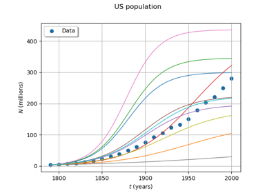
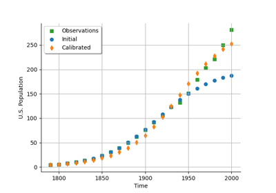
Data class for the logistic model.
In the physical model, the inputs and parameters are ordered as presented in the next table. Notice that there are no parameters in the physical model.
Index
Input variable
0
t1
1
t2
…
…
21
t22
22
a
23
c
Examples
>>> from openturns.usecases import logistic_model
>>> # Load the logistic model
>>> lm = logistic_model.LogisticModel()
>>> print(lm.data[:5])
    [ Time            U.S. Population ]
0 : [ 1790               3.9          ]
1 : [ 1800               5.3          ]
2 : [ 1810               7.2          ]
3 : [ 1820               9.6          ]
4 : [ 1830              13            ]
>>> print("Inputs:", lm.model.getInputDescription())
Inputs: [t0,t1,t2,t3,t4,t5,t6,t7,t8,t9,t10,t11,t12,t13,t14,t15,t16,t17,t18,t19,t20,t21,a,c]#24
>>> print("Outputs:", lm.model.getOutputDescription())
Outputs: [z0,z1,z2,z3,z4,z5,z6,z7,z8,z9,z10,z11,z12,z13,z14,z15,z16,z17,z18,z19,z20,z21]#22
- Attributes:
- t0float, optional
Initial time. The default is 1790.
- y0float, optional
Initial population (at t0). The default is 3.9e6.
- afloat, optional
8Parameter of the model. The default is 0.03134.
- bfloat, optional
Parameter of the model. The default is 1.5887e-10.
- populationFactorfloat, optional
The multiplication factor to scale the population. The default is 1.0e6.
- distY0
Normaldistribution ot.Normal(y0, 0.1 * y0)
- distA
Normaldistribution ot.Normal(a, 0.3 * a)
- distB
Normaldistribution ot.Normal(b, 0.3 * b)
- distX
ComposedDistribution The joint distribution of the input parameters.
- model
PythonFunction The logistic model of growth. The input has input dimension 24 and output dimension 22. More precisely, we have
 and
and  .
.- data
Sampleof size 22 and dimension 2 A data set containing 22 dates from 1790 to 2000. First marginal represents dates and second marginal the population in millions.
- __init__(t0=1790.0, y0=3900000.0, a=0.03134, b=1.5887e-10, populationFactor=1000000.0)