Note
Go to the end to download the full example code.
Kriging the cantilever beam model using HMAT
In this example, we create a Kriging metamodel of the cantilever beam. We use a squared exponential covariance kernel for the Gaussian process. In order to estimate the hyper-parameters, we use a design of experiments of size is 20.
Definition of the model
from openturns.usecases import cantilever_beam
import openturns as ot
import openturns.viewer as viewer
from matplotlib import pylab as plt

ot.Log.Show(ot.Log.NONE)
We load the cantilever beam use case :
cb = cantilever_beam.CantileverBeam()
We define the function which evaluates the output depending on the inputs.
model = cb.model
Then we define the distribution of the input random vector.
dim = cb.dim  # number of inputs
myDistribution = cb.distribution
Create the design of experiments
We consider a simple Monte-Carlo sample as a design of experiments. This is why we generate an input sample using the getSample method of the distribution. Then we evaluate the output using the model function.
sampleSize_train = 20
X_train = myDistribution.getSample(sampleSize_train)
Y_train = model(X_train)
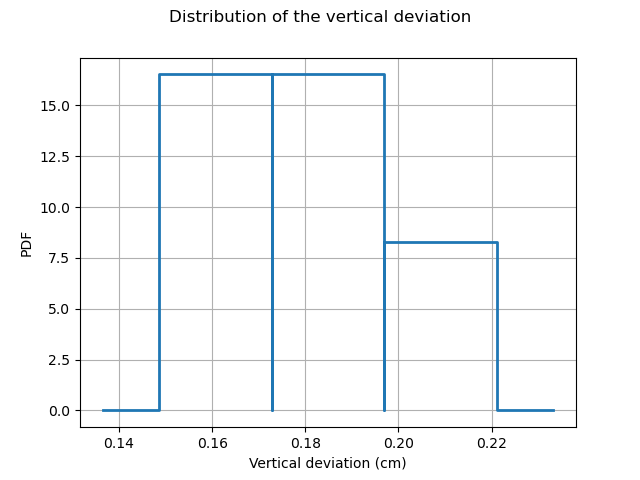
The following figure presents the distribution of the vertical deviations Y on the training sample. We observe that the large deviations occur less often.
histo = ot.HistogramFactory().build(Y_train).drawPDF()
histo.setXTitle("Vertical deviation (cm)")
histo.setTitle("Distribution of the vertical deviation")
histo.setLegends([""])
view = viewer.View(histo)
Create the metamodel
We rely on H-Matrix approximation for accelerating the evaluation. We change default parameters (compression, recompression) to higher values. The model is less accurate but very fast to build & evaluate.
ot.ResourceMap.SetAsString("KrigingAlgorithm-LinearAlgebra", "HMAT")
ot.ResourceMap.SetAsScalar("HMatrix-AssemblyEpsilon", 1e-5)
ot.ResourceMap.SetAsScalar("HMatrix-RecompressionEpsilon", 1e-4)
In order to create the Kriging metamodel, we first select a constant trend with the ConstantBasisFactory class. Then we use a squared exponential covariance kernel. The SquaredExponential kernel has one amplitude coefficient and 4 scale coefficients. This is because this covariance kernel is anisotropic : each of the 4 input variables is associated with its own scale coefficient.
basis = ot.ConstantBasisFactory(dim).build()
covarianceModel = ot.SquaredExponential(dim)
Typically, the optimization algorithm is quite good at setting sensible optimization bounds. In this case, however, the range of the input domain is extreme.
print("Lower and upper bounds of X_train:")
print(X_train.getMin(), X_train.getMax())
Lower and upper bounds of X_train:
[6.50131e+10,262.222,2.5196,1.309e-07] [7.07581e+10,340.736,2.5983,1.6534e-07]
We need to manually define sensible optimization bounds. Note that since the amplitude parameter is computed analytically (this is possible when the output dimension is 1), we only need to set bounds on the scale parameter.
scaleOptimizationBounds = ot.Interval(
    [1.0, 1.0, 1.0, 1.0e-10], [1.0e11, 1.0e3, 1.0e1, 1.0e-5]
)
Finally, we use the KrigingAlgorithm class to create the Kriging metamodel. It requires a training sample, a covariance kernel and a trend basis as input arguments. We need to set the initial scale parameter for the optimization. The upper bound of the input domain is a sensible choice here. We must not forget to actually set the optimization bounds defined above.
covarianceModel.setScale(X_train.getMax())
algo = ot.KrigingAlgorithm(X_train, Y_train, covarianceModel, basis)
algo.setOptimizationBounds(scaleOptimizationBounds)
The run method has optimized the hyperparameters of the metamodel.
We can then print the constant trend of the metamodel, which have been estimated using the least squares method.
algo.run()
result = algo.getResult()
krigingMetamodel = result.getMetaModel()
The getTrendCoefficients method returns the coefficients of the trend.
print(result.getTrendCoefficients())
[0.184941]
We can also print the hyperparameters of the covariance model, which have been estimated by maximizing the likelihood.
result.getCovarianceModel()
Validate the metamodel
We finally want to validate the Kriging metamodel. This is why we generate a validation sample with size 100 and we evaluate the output of the model on this sample.
sampleSize_test = 100
X_test = myDistribution.getSample(sampleSize_test)
Y_test = model(X_test)
The MetaModelValidation classe makes the validation easy. To create it, we use the validation samples and the metamodel.
val = ot.MetaModelValidation(Y_test, krigingMetamodel(X_test))
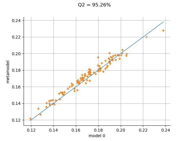
The computePredictivityFactor computes the Q2 factor.
R2 = val.computeR2Score()[0]
print(R2)
0.9526427539844872
The residuals are the difference between the model and the metamodel.
r = val.getResidualSample()
graph = ot.HistogramFactory().build(r).drawPDF()
graph.setXTitle("Residuals (cm)")
graph.setTitle("Distribution of the residuals")
graph.setLegends([""])
view = viewer.View(graph)
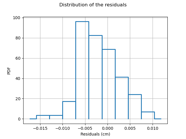
We observe that the negative residuals occur with nearly the same frequency of the positive residuals: this is a first sign of good quality.
The drawValidation method allows one to compare the observed outputs and the metamodel outputs.
sphinx_gallery_thumbnail_number = 3
graph = val.drawValidation()
graph.setTitle("R2 = %.2f%%" % (100 * R2))
view = viewer.View(graph)

plt.show()
Reset default settings
ot.ResourceMap.Reload()