Note
Go to the end to download the full example code.
Create a gaussian process from a cov. model using HMatrix
In this basic example we build a gaussian process from its covariance model and use the HMatrix method as a sampling method. Several methods and parameters are presented to set the HMatrix compression. This is an advanced topic and we should highlight key ideas only in this example.
import openturns as ot
import openturns.viewer as viewer
from matplotlib import pylab as plt

# ot.Log.Show(ot.Log.NONE)
Definition of the covariance model
We define our Gaussian process from its covariance model. We consider a Gaussian kernel with the following parameters.
dimension = 1
amplitude = [1.0] * dimension
scale = [1] * dimension
covarianceModel = ot.GeneralizedExponential(scale, amplitude, 2)
We define the time grid on which we want to sample the Gaussian process.
tmin = 0.0
step = 0.01
n = 10001
timeGrid = ot.RegularGrid(tmin, step, n)
Finally we define the Gaussian process.
process = ot.GaussianProcess(covarianceModel, timeGrid)
print(process)
GaussianProcess(trend=[x0]->[0.0], covariance=GeneralizedExponential(scale=[1], amplitude=[1], p=2))
Basics on the HMatrix algebra
The HMatrix framework uses efficient linear algebra techniques to speed-up the (Cholesky) factorization of the covariance matrix. This method can be tuned with several parameters. We should concentrate on the easiest ones.
We set the sampling method to HMAT (default is the classical/dense case).
process.setSamplingMethod(ot.GaussianProcess.HMAT)
The HMatrix framework uses an algebraic algorithm to compress sub-blocks of the matrix. Several algorithms are available and can be set from the ResourceMap key.
ot.ResourceMap.SetAsString("HMatrix-CompressionMethod", "AcaRandom")
There are two threshold used in the HMatrix framework. The AssemblyEpsilon is the most important one.
ot.ResourceMap.SetAsScalar("HMatrix-AssemblyEpsilon", 1e-7)
ot.ResourceMap.SetAsScalar("HMatrix-RecompressionEpsilon", 1e-7)
Process sampling
We eventually draw samples of this covariance model.
sample = process.getSample(6)
graph = sample.drawMarginal(0)
view = viewer.View(graph)
plt.show()
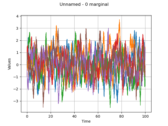
We notice here that we are able to sample the covariance model over a mesh of size 10000, which is usually tricky on a laptop. This is mainly due to the compression.
Reset default settings
ot.ResourceMap.Reload()
Total running time of the script: (0 minutes 2.338 seconds)