Note

Go to the end to download the full example code.

Draw a field¶

In this example, we show the different ways of drawing a Field that is a realization of a process.

We consider the following fields:

Case 1: A field defined on a 2-d mesh with 2-d values,
Case 2: A field defined on a 2-d mesh with scalar values,
Case 3: A field defined on a 1-d mesh with 2-d values,
Case 4: A field defined on a 1-d mesh with scalar values.

import openturns as ot
import openturns.viewer as otv

# sphinx_gallery_thumbnail_number = 2

Case 1: A field defined on a 2-d mesh with 2-d values¶

We consider a normal process defined on $\cD = [0,1]^2$ , with 2-d output values, defined by a covariance function which is a TensorizedCovarianceModel built as the tensorization of two MaternModel covariance functions. The domain $\cD$ is discretized by a regular grid, using the class IntervalMesher.

cov_model = ot.TensorizedCovarianceModel([ot.MaternModel([0.1] * 2, [0.01], 2.5)] * 2)
mesh = ot.IntervalMesher([30] * 2).build(ot.Interval([0.0] * 2, [1.0] * 2))
normal_proc = ot.GaussianProcess(cov_model, mesh)
field = normal_proc.getRealization()

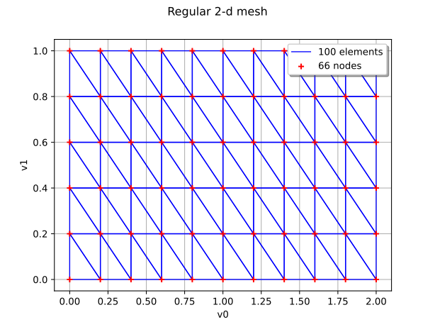
We first draw the field with arrows fixed on each vertex of the mesh.

g_1 = field.draw()
g_1.setTitle(r"A field on 2-d mesh and 2-d values")
g_1.setXTitle(r"$x_0$")
g_1.setYTitle(r"$x_1$")

In order to change the arrows, we can modify the ResourceMap keys associated to the class Field.

ot.ResourceMap.SetAsScalar("Field-ArrowRatio", 0.05)
ot.ResourceMap.SetAsScalar("Field-ArrowScaling", 0.8)
g_2 = field.draw()

g_2.setTitle("The same field with other arrows parameters")
g_2.setXTitle(r"$x_0$")
g_2.setYTitle(r"$x_1$")

We can compare both figures.

grid = ot.GridLayout(1, 2)
grid.setGraph(0, 0, g_1)
grid.setGraph(0, 1, g_2)
view = otv.View(grid)

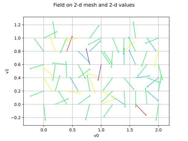
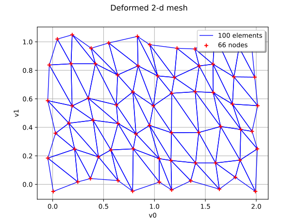
, A field on 2-d mesh and 2-d values, The same field with other arrows parameters

We can also use the output values to deform the initial mesh and draw the deformed mesh. First, we recover the default values of the ResourceMap keys.

ot.ResourceMap.SetAsScalar("Field-ArrowRatio", 0.01)
ot.ResourceMap.SetAsScalar("Field-ArrowScaling", 1)
deformed_field = field.asDeformedMesh()
g_def = deformed_field.draw()
g_def.setTitle("The same field as deformed mesh")
g_def.setXTitle(r"$x_0$")
g_def.setYTitle(r"$x_1$")
g_def.setLegendPosition("")

We can compare both figures.

grid = ot.GridLayout(1, 2)
grid.setGraph(0, 0, g_1)
grid.setGraph(0, 1, g_def)
view = otv.View(grid)

, A field on 2-d mesh and 2-d values, The same field as deformed mesh

Case 2: A field defined on a 2-d mesh with scalar values¶

We consider a normal process defined on $\cD = [0,1]^2$ , with scalar output values, defined by a covariance function which is a MaternModel. The domain $\cD$ is discretized by a regular grid, using the class IntervalMesher.

cov_model = ot.MaternModel([0.15] * 2, [0.01], 2.5)
mesh = ot.IntervalMesher([35] * 2).build(ot.Interval([0.0] * 2, [1.0] * 2))
normal_proc = ot.GaussianProcess(cov_model, mesh)
field = normal_proc.getRealization()

We draw the field by filling each cell of the mesh with a color.

g_1 = field.draw()
g_1.setTitle("A field on 2-d mesh  and scalar values")
g_1.setXTitle(r"$x_0$")
g_1.setYTitle(r"$x_1$")

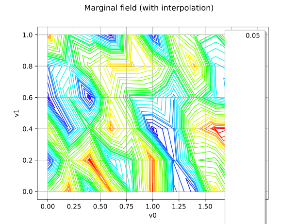
We can also draw iso-value lines of the output values using interpolation.

g_2 = field.drawMarginal(0, True)
g_2.setTitle("A field on 2-d mesh and scalar values")
g_2.setXTitle(r"$x_0$")
g_2.setYTitle(r"$x_1$")
g_2.setLegendPosition("")

We can compare both figures.

grid = ot.GridLayout(1, 2)
grid.setGraph(0, 0, g_1)
grid.setGraph(0, 1, g_2)
view = otv.View(grid)

, A field on 2-d mesh and scalar values, A field on 2-d mesh and scalar values

Case 3: A field defined on a 1-d mesh with 2-d values¶

We consider a RandomWalk process which distribution is the normal distribution of dimension 2 with zero mean and identity covariance matrix. The process is defined on $\cD = [0,1]$ which is discretized by a regular grid, using the class RegularGrid.

dist_rw = ot.Normal(2)
origin = dist_rw.getMean()
N = 10000
step = 1.0 / N
mesh = ot.RegularGrid(0, step, N)
rw_process = ot.RandomWalk(origin, dist_rw, mesh)
field = rw_process.getRealization()

We draw the field by interpolating the output vectors.

g = field.draw()
g.setTitle("A 2-d random walk field")
g.setXTitle(r"$x_0$")
g.setYTitle(r"$x_1$")
view = otv.View(g)

Case 4: A field defined on a 1-d mesh with scalar values¶

We consider a normal process defined on $\cD = [0,1]$ , with scalar output values, defined by a covariance function which is a MaternModel. The domain $\cD$ is discretized by a regular grid, using IntervalMesher. This process is stationary.

cov_model = ot.MaternModel([0.05], [0.01], 2.5)
mesh = ot.IntervalMesher([1000]).build(ot.Interval(0.0, 1.0))
normal_proc = ot.GaussianProcess(cov_model, mesh)
field = normal_proc.getRealization()

We draw its trajectory without interpolating the output values.

g_1 = field.draw()
g_1.setTitle("A field on 1-d mesh and scalar values - Stationary process")
g_1.setXTitle(r"$x_0$")
g_1.setYTitle(r"$x_1$")

We can also interpolate the output values.

g_2 = field.drawMarginal(0, True)
g_2.setTitle("The same field with interpolation")
g_2.setXTitle(r"$x_0$")
g_2.setYTitle(r"$x_1$")
g_2.setLegendPosition("")

We can compare both figures.

grid = ot.GridLayout(1, 2)
grid.setGraph(0, 0, g_1)
grid.setGraph(0, 1, g_2)
view = otv.View(grid)

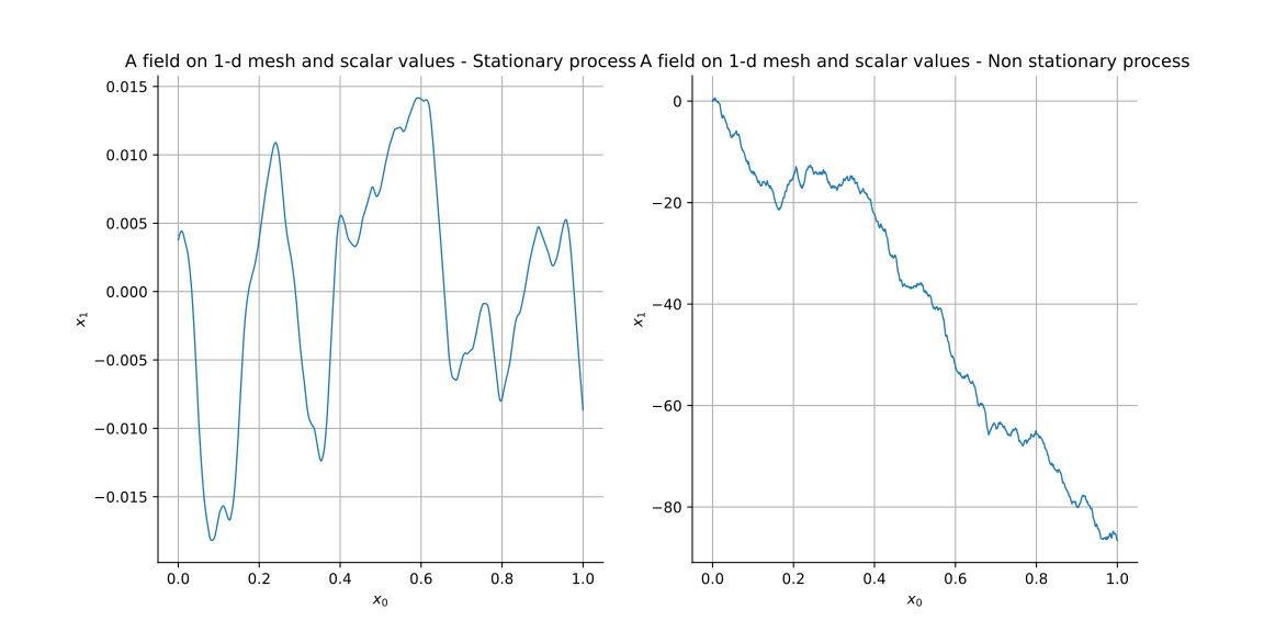
, A field on 1-d mesh and scalar values - Stationary process, The same field with interpolation

We consider now a normal process which is not stationary. We use the FractionalBrownianMotionModel:

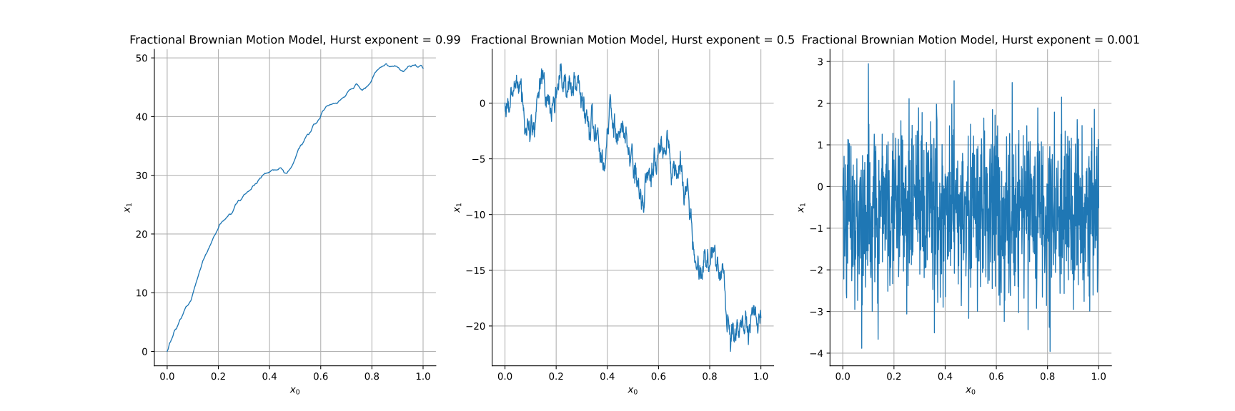
when the Hurst exponent is close to 1, the trajectory is smooth,
when the Hurst exponent is equal to 1/2, the trajectory is Brownian motion (Wiener process),
when the Hurst exponent is close to 0, the process tends to a White noise process.

scale = 0.01
amplitude = 1.5
hurst_exponent = 0.75
cov_model = ot.FractionalBrownianMotionModel(scale, amplitude, hurst_exponent)
mesh = ot.IntervalMesher([1000]).build(ot.Interval(0.0, 1.0))
normal_proc = ot.GaussianProcess(cov_model, mesh)
field = normal_proc.getRealization()
g_3 = field.drawMarginal(0, True)
g_3.setTitle("A field on 1-d mesh and scalar values - Non stationary process")
g_3.setXTitle(r"$x_0$")
g_3.setYTitle(r"$x_1$")

We can compare both processes.

grid = ot.GridLayout(1, 2)
g_2.setTitle("A field on 1-d mesh and scalar values - Stationary process")
grid.setGraph(0, 0, g_2)
grid.setGraph(0, 1, g_3)
view = otv.View(grid)

, A field on 1-d mesh and scalar values - Stationary process, A field on 1-d mesh and scalar values - Non stationary process

We draw here a trajectory from a FractionalBrownianMotionModel with different Hurst exponent.

grid = ot.GridLayout(1, 3)
hurst_exponent_list = [0.99, 0.50, 0.001]
for index, hurst_exponent in enumerate(hurst_exponent_list):
    cov_model = ot.FractionalBrownianMotionModel(scale, amplitude, hurst_exponent)
    normal_proc = ot.GaussianProcess(cov_model, mesh)
    field = normal_proc.getRealization()
    g = field.drawMarginal(0, True)
    g.setTitle(
        r"Fractional Brownian Motion Model, Hurst exponent = " + str(hurst_exponent)
    )
    g.setXTitle(r"$x_0$")
    g.setYTitle(r"$x_1$")
    grid.setGraph(0, index, g)
view = otv.View(grid)

, Fractional Brownian Motion Model, Hurst exponent = 0.99, Fractional Brownian Motion Model, Hurst exponent = 0.5, Fractional Brownian Motion Model, Hurst exponent = 0.001

Display all figures

otv.View.ShowAll()

OpenTURNS

An Open source initiative for the Treatment of Uncertainties, Risks'N Statistics

Table of Contents

Previous topic

Next topic

This Page

Draw a field¶

Case 1: A field defined on a 2-d mesh with 2-d values¶

Case 2: A field defined on a 2-d mesh with scalar values¶

Case 3: A field defined on a 1-d mesh with 2-d values¶

Case 4: A field defined on a 1-d mesh with scalar values¶