 OpenTURNS
DivFreeModel
(Source code, svg)
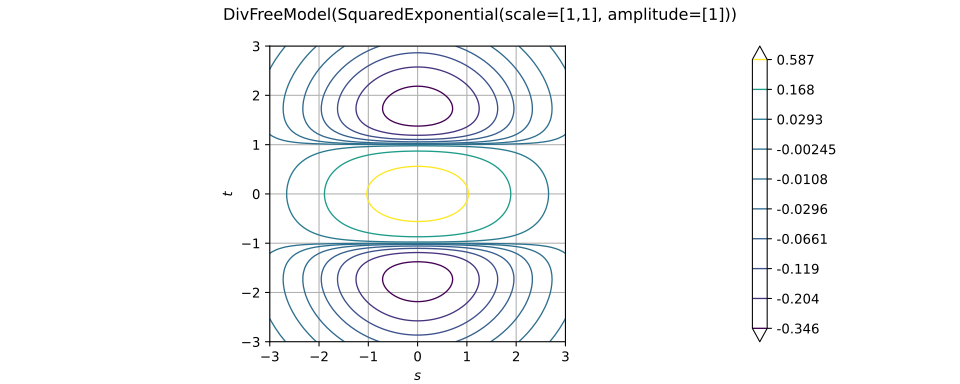
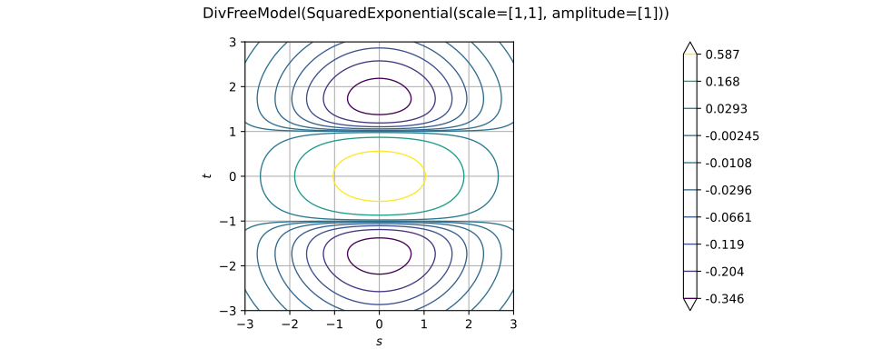
- class DivFreeModel(*args)
Divergence-free covariance model.
Warning
This class is experimental and likely to be modified in future releases. To use it, import the
openturns.experimentalsubmodule.This class builds a matrix-valued divergence-free covariance model from a scalar covariance model
 , as described in [scheuerer2012].
Let
 be a scalar covariance
model, and let
 be the matrix of mixed
second derivatives:

The divergence-free covariance model is defined as:

The resulting model has input dimension
 and output dimension
 , with
 . If the
underlying scalar model has
 regularity, the
associated random vector field has divergence-free sample paths almost surely.
The model is defined for input dimensions
 . For
 the model has been conjectured to work but only proven
for
 [scheuerer2012].
- Parameters:
- model
CovarianceModel A scalar covariance model
.
- model
Methods
activateAmplitude(isAmplitudeActive)Activate/deactivate the amplitude parameters.
activateNuggetFactor(isNuggetFactorActive)Activate/deactivate the nugget factor.
activateScale(isScaleActive)Activate/deactivate the scale parameters.
computeAsScalar(*args)Compute the covariance function for a scalar model.
computeCrossCovariance(*args)Compute the covariance function on two given meshes.
discretize(*args)Discretize the covariance function on a given mesh.
discretizeAndFactorize(*args)Discretize and factorize the covariance function on a given mesh.
Discretize and factorize the covariance function on a given mesh using HMatrix.
Discretize and factorize the covariance function on a given mesh using HODLRMatrix.
discretizeHMatrix(*args)Discretize the covariance function on a given mesh using HMatrix.
discretizeHODLRMatrix(*args)Discretize the covariance function on a given mesh using HODLRMatrix.
discretizeRow(vertices, p)Discretize the covariance function on a given mesh for a specific row.
draw(*args)Draw a specific component of the covariance model with input dimension 1.
fourthOrderPartial(s, t)Compute the fourth-order spatial derivatives of the
 output component of the covariance function.
Accessor to the active parameter set.
Get the amplitude parameter
 of the covariance function.
Accessor to the object's name.
Accessor to the underlying scalar covariance model.
Get the full parameters of the covariance function.
Get the description of the full parameters of the covariance function.
Get the input dimension of the covariance function.
getMarginal(*args)Get the marginal covariance model.
getName()Accessor to the object's name.
Accessor to the nugget factor.
Get the spatial correlation matrix
 of the covariance function.
Get the output dimension of the covariance function.
Get the values of the active parameters of the covariance function.
Get the description of the active parameters of the covariance function.
getScale()Get the scale parameter
 of the covariance function.
hasName()Test if the object is named.
Test whether the model is diagonal.
Accessor to the parallel flag.
Test whether the model is stationary.
parameterGradient(s, t)Compute the gradient of the covariance function with respect to the active parameters.
parameterHessian(s, t)Compute the mixed parameter-spatial Hessian of the
output component of the covariance function.partialGradient(s, t)Compute the gradient of the covariance function with respect to the first index
 .
partialHessian(s, t)Compute the Hessian of the
output component of the covariance function with respect to the first index .setActiveParameter(active)Accessor to the active parameter set.
setAmplitude(amplitude)Set the amplitude parameter
of the covariance function.setFullParameter(parameter)Set the full parameters of the covariance function.
setName(name)Accessor to the object's name.
setNuggetFactor(nuggetFactor)Set the nugget factor for the variance of the observation error.
setOutputCorrelation(correlation)Set the spatial correlation matrix
of the covariance function.setParameter(parameter)Set the values of the active parameters of the covariance function.
setScale(scale)Set the scale parameter
of the covariance function.thirdOrderPartial(s, t)Compute the third-order spatial derivatives of the
output component of the covariance function.Examples
>>> import openturns as ot
>>> import openturns.experimental as otexp
>>> scale = [1.0, 1.5]
>>> amplitude = [1.0]
>>> cov = ot.SquaredExponential(scale, amplitude)
>>> divFreeCov = otexp.DivFreeModel(cov)
>>> print(divFreeCov.getInputDimension())
2
>>> print(divFreeCov.getOutputDimension())
2
>>> s = [0.5, 0.3]
>>> t = [0.1, 0.2]
>>> print(divFreeCov(s, t))
[[ 0.407544  0.0163745 ]
 [ 0.0163745 0.773696  ]]
- __init__(*args)
- activateAmplitude(isAmplitudeActive)
Activate/deactivate the amplitude parameters.
In the context of kriging, defines whether the amplitude parameters should be tuned.
- Parameters:
- isAmplitudeActivebool
If
True, all the amplitude parameters are tuned. IfFalse, none of them is tuned.
- activateNuggetFactor(isNuggetFactorActive)
Activate/deactivate the nugget factor.
In the context of kriging, defines whether the nugget factor should be tuned.
- Parameters:
- isNuggetFactorActivebool
If
True(respectivelyFalse), the nugget factor is (respectively is not) tuned.
- activateScale(isScaleActive)
Activate/deactivate the scale parameters.
In the context of kriging, defines whether the scale parameters should be tuned.
- Parameters:
- isScaleActivebool
If
True, all the scale parameters are tuned. IfFalse, none of them is tuned.
- computeAsScalar(*args)
Compute the covariance function for a scalar model.
- Available usages:
computeAsScalar(s, t)
computeAsScalar(tau)
- Parameters:
- s, tfloat or sequence of float
Multivariate index
 .
Scalars are accepted only if
 .
- taufloat or sequence of float
Multivariate index
 .
A scalar is accepted only if .
- Returns:
- covariancefloat
Covariance value.
Notes
The method makes sense only if the dimension of the process is
 , in which case the covariance matrix
 reduces to the scalar covariance
 .
In the second usage, the covariance model must be stationary. We then note
 for
 , as this quantity does not
depend on .
- computeCrossCovariance(*args)
Compute the covariance function on two given meshes.
- Parameters:
- Returns:
- crossCovariance
Matrix Cross-covariance matrix of size
 , where
 and
 are the numbers of vertices in
firstVertices and secondVertices.
- crossCovariance
Notes
The cross-covariance matrix is the evaluation of the covariance model on both firstVertices and secondVertices.
The result is a
matrix, i.e. a block matrix
whose  block is
 , where
 are the points of
firstVertices and
 are the points of
secondVertices. When , this is the
 matrix with entries
.
- discretize(*args)
Discretize the covariance function on a given mesh.
- Parameters:
- where
MeshorRegularGridorSample Container of the discretization vertices.
- where
- Returns:
- covarianceMatrix
CovarianceMatrix Covariance matrix
 of size
 , where
 is the number of vertices.
- covarianceMatrix
Notes
Let
 be the vertices of the given
mesh. The method returns the block covariance matrix

- discretizeAndFactorize(*args)
Discretize and factorize the covariance function on a given mesh.
- Parameters:
- where
MeshorRegularGridorSample Container of the discretization vertices.
- where
- Returns:
- choleskyFactor
TriangularMatrix Lower triangular Cholesky factor
 of the covariance
matrix, of size , such that
 , where
is the number of vertices.
- choleskyFactor
Notes
This method discretizes the model on the given
Mesh,RegularGridorSamplewith thediscretize()method and returns its Cholesky factor.
- discretizeAndFactorizeHMatrix(*args)
Discretize and factorize the covariance function on a given mesh using HMatrix.
- Parameters:
- where
MeshorRegularGridorSample Container of the discretization vertices.
- hmatParam
HMatrixParameters Parameter values for the HMatrix.
- where
- Returns:
- choleskyFactor
HMatrix Lower triangular Cholesky factor
of the covariance
matrix, of size , such that
when the
factorization method is LLt(default), stored in hierarchical format (H-Matrix). With theLUorLDLtmethod, the result holds the factorization computed by that method instead.
- choleskyFactor
Notes
This method is similar to the
discretizeAndFactorize()method. It requires that the library has been compiled with HMAT support. It is helpful for very large discretization sizes because it compresses the data.
- discretizeAndFactorizeHODLRMatrix(*args)
Discretize and factorize the covariance function on a given mesh using HODLRMatrix.
- Parameters:
- where
MeshorRegularGridorSample Container of the discretization vertices.
- hodlrParam
HODLRMatrixParameters Parameter values for the HODLR matrix.
- where
- Returns:
- choleskyFactor
HODLRMatrix Lower triangular Cholesky factor
of the covariance
matrix, of size , such that
, stored in
hierarchical format (HODLR), where is the number of
vertices.
- choleskyFactor
Notes
This method is similar to the
discretizeAndFactorize()method, but stores the result in aHODLRMatrixinstead of a denseTriangularMatrix. It does not require any external library. It is helpful for very large discretization sizes because it compresses the data.
- discretizeHMatrix(*args)
Discretize the covariance function on a given mesh using HMatrix.
- Parameters:
- where
MeshorRegularGridorSample Container of the discretization vertices.
- hmatParam
HMatrixParameters Parameter values for the HMatrix.
- where
- Returns:
- covarianceMatrix
HMatrix Covariance matrix
of size , stored in
hierarchical format (H-Matrix), where is the number of
vertices.
- covarianceMatrix
Notes
This method is similar to the
discretize()method. It requires that the library has been compiled with HMAT support. It is helpful for very large discretization sizes because it compresses the data.
- discretizeHODLRMatrix(*args)
Discretize the covariance function on a given mesh using HODLRMatrix.
- Parameters:
- where
MeshorRegularGridorSample Container of the discretization vertices.
- hodlrParam
HODLRMatrixParameters Parameter values for the HODLR matrix.
- where
- Returns:
- covarianceMatrix
HODLRMatrix Covariance matrix
of size , stored in
hierarchical format (HODLR), where is the number of
vertices.
- covarianceMatrix
Notes
This method is similar to the
discretize()method, but stores the result in aHODLRMatrixinstead of a denseCovarianceMatrix. It is helpful for very large discretization sizes because it compresses the data. It does not require any external library. The result must be factorized with thefactorize()method before being used bysolve()orlogDeterminant().
- discretizeRow(vertices, p)
Discretize the covariance function on a given mesh for a specific row.
- Parameters:
- vertices
Sample Container of the discretization vertices
 .
- pint,

Row index of the covariance matrix to discretize.
- vertices
- Returns:
- result
Sample Sample of size
 and dimension
, whose
 -th block of
rows contains the covariance matrix
 , for
 .
- result
Notes
When
, the result is a sample of size
and dimension 1 with entries
 .
- draw(*args)
Draw a specific component of the covariance model with input dimension 1.
- Parameters:
- rowIndexint,

Row index of the component to draw. Default value is 0.
- columnIndexint,

Column index of the component to draw. Default value is 0.
- tMinfloat
Lower bound
 of the range over which the model is
plotted. Default value is
CovarianceModel-DefaultTMininResourceMap.- tMaxfloat
Upper bound
 of the range over which the model is
plotted. Default value is
CovarianceModel-DefaultTMaxinResourceMap.- pointNumberint,

Number of points used to discretize the range
 . Default value is
CovarianceModel-DefaultPointNumberinResourceMap.- asStationarybool
If
True, the model is plotted as a function of the lag when the model is stationary. If
False, it is plotted as a function of . Default value is
True.- correlationFlagbool
If
True, the model is plotted as a correlation function. IfFalse, it is plotted as a covariance function. Default value isFalse.
- rowIndexint,
- Returns:
- graph
Graph A graph containing a unique curve if asStationary is
Trueand if the model is actually stationary, or the iso-values of the model otherwise.
- graph
Notes
This method requires
.
- fourthOrderPartial(s, t)
Compute the fourth-order spatial derivatives of the
output component of the covariance function.- Parameters:
- s, tfloat or sequence of float
Multivariate index
.
Each vector has dimension .
Scalars are accepted only if .
- Returns:
- fourth
Point Fourth-order derivatives of the
output component
 with respect to
 , stored as a flat point of
size
 ; for
 , index
 holds
 .
- fourth
- getActiveParameter()
Accessor to the active parameter set.
In the context of kriging, it allows one to choose which hyperparameters are tuned.
- Returns:
- active
Indices Indices of the active parameters among the full parameter vector.
- active
- getAmplitude()
Get the amplitude parameter
of the covariance function.- Returns:
- amplitude
Point Amplitude parameter
 . Its components are positive.
- amplitude
- getClassName()
Accessor to the object’s name.
- Returns:
- class_namestr
The object class name (object.__class__.__name__).
- getCovarianceModel()
Accessor to the underlying scalar covariance model.
- Returns:
- model
CovarianceModel The underlying scalar covariance model.
- model
- getFullParameter()
Get the full parameters of the covariance function.
- Returns:
- parameter
Point Full parameter vector, of size at least
 .
In the base class, its components are, in order, the scale vector
, the nugget factor
 , the amplitude vector
and the lower triangle of the spatial
correlation matrix . Models may append model-specific
parameters.
- parameter
- getFullParameterDescription()
Get the description of the full parameters of the covariance function.
- Returns:
- description
Description Description of the full parameter vector, in the order returned by
getFullParameter().
- description
- getInputDimension()
Get the input dimension of the covariance function.
- Returns:
- inputDimensionint
Dimension
of the index domain  .
It is such that
 .
- getMarginal(*args)
Get the marginal covariance model.
- Parameters:
- indexint or sequence of int
Index or indices of the components of the process to keep.
- Returns:
- marginal
CovarianceModel Covariance model restricted to the selected components.
- marginal
- getName()
Accessor to the object’s name.
- Returns:
- namestr
The name of the object.
- getNuggetFactor()
Accessor to the nugget factor.
The nugget factor
is a dimensionless
nonnegative parameter which models a noise on the observed values of the
process. At  , it replaces the covariance
matrix
 by
 .
- Returns:
- nuggetFactorfloat
Nugget factor
 .
- getOutputCorrelation()
Get the spatial correlation matrix
of the covariance function.- Returns:
- spatialCorrelation
CorrelationMatrix Spatial correlation matrix
 of size
 .
- spatialCorrelation
- getOutputDimension()
Get the output dimension of the covariance function.
- Returns:
- outputDimensionint
Dimension
of the process  .
It is such that
 .
- getParameter()
Get the values of the active parameters of the covariance function.
- Returns:
- parameter
Point Values of the
 active parameters, in the order given by
getParameterDescription().
- parameter
Notes
The active parameters are selected by
setActiveParameter()among the full parameters returned bygetFullParameter().
- getParameterDescription()
Get the description of the active parameters of the covariance function.
- Returns:
- descriptionParam
Description Description of the active parameters, i.e. the components of
getFullParameterDescription()selected bygetActiveParameter().
- descriptionParam
- getScale()
Get the scale parameter
of the covariance function.- Returns:
- scale
Point Scale parameter
 used in the covariance function.
Its components are positive.
For
IsotropicCovarianceModel, the scale has a single component.
- scale
- hasName()
Test if the object is named.
- Returns:
- hasNamebool
True if the name is not empty.
- isDiagonal()
Test whether the model is diagonal.
- Returns:
- isDiagonalbool
Trueif the covariance matrix is diagonal, i.e.
- isParallel()
Accessor to the parallel flag.
- Returns:
- isParallelbool
Whether the object is considered thread-safe.
- isStationary()
Test whether the model is stationary.
- Returns:
- isStationarybool
Trueif the covariance function is invariant by translation.
Notes
The covariance function is stationary when it depends only on the lag
 :

In that case, we note
 for
 .
- parameterGradient(s, t)
Compute the gradient of the covariance function with respect to the active parameters.
- Parameters:
- s, tfloat or sequence of float
Multivariate index
.
Each vector has dimension .
Scalars are accepted only if .
- Returns:
- gradient
Matrix Gradient of the covariance function
with respect to the
active parameters
 , in the order given by
getParameterDescription(). Its size is .
For
 and
 , row
 and column
 hold
 .
The matrix
 associated with each row is thus flattened column by column.
- gradient
- parameterHessian(s, t)
Compute the mixed parameter-spatial Hessian of the
output component of the covariance function.- Parameters:
- s, tfloat or sequence of float
Multivariate index
.
Each vector has dimension .
Scalars are accepted only if .
- Returns:
- hessian
Matrix Derivatives of the partial Hessian
 of the output component
with respect to the active parameters
, in the order given by
getParameterDescription(). Its size is .
For and
 , row and column
 hold
 .
The
 partial Hessian
associated with each row is thus flattened column by column.
- hessian
- partialGradient(s, t)
Compute the gradient of the covariance function with respect to the first index
.- Parameters:
- s, tfloat or sequence of float
Multivariate index
.
Each vector has dimension .
Scalars are accepted only if .
- Returns:
- gradient
Matrix Gradient of the covariance function
with respect to
. Its size is
 .
For
 and
, row
 and column
hold
 .
The matrix
 associated with each row is thus flattened column by column.
- gradient
- partialHessian(s, t)
Compute the Hessian of the
output component of the covariance function with respect to the first index .- Parameters:
- s, tfloat or sequence of float
Multivariate index
.
Each vector has dimension .
Scalars are accepted only if .
- Returns:
- hessian
SymmetricMatrix Hessian of the
output component
with respect to
. Its size is
; entry  holds
.
The other output components are not differentiated.
- hessian
- setActiveParameter(active)
Accessor to the active parameter set.
This method defines which hyperparameters are tuned.
- Parameters:
- activesequence of int
Indices of the active parameters among the full parameter vector.
Notes
The indices refer to the full parameter vector returned by
getFullParameter(). In order to get the position of a parameter known by its name, first call the methodgetFullParameterDescription()and then use the index method of the returnedDescription, as shown in the following example.Examples
For example, we create a
MaternModelcovariance model. By default, only the scale and the amplitude parameters are active and will be estimated. We want to add the estimation of the parameter.
>>> import openturns as ot
>>> covModel = ot.MaternModel()
We get the default active parameters description: we can see that the
parameter is not included in the list.>>> covModel.getParameterDescription() [scale_0,amplitude_0]
We now get the active parameters. The parameter
is not in the
list.>>> active = covModel.getActiveParameter() >>> print(active) [0,2]
We want to search the index associated to the parameter
in the
full list of the parameters indices.>>> activeDesc = covModel.getFullParameterDescription() >>> print(activeDesc) [scale_0,nuggetFactor,amplitude_0,nu] >>> index = activeDesc.index('nu') >>> print(index) 3
Now, we add the index of
in the initial list of active
parameters. We sort the active indices by increasing order. Then we update
the list of the active parameters.>>> active = covModel.getActiveParameter() >>> active.add(index) >>> covModel.setActiveParameter(sorted(active))
Check that the parameter
is in the active parameters list!>>> covModel.getActiveParameter() [0,2,3]
>>> covModel.getFullParameterDescription()
[scale_0,nuggetFactor,amplitude_0,nu]
- setAmplitude(amplitude)
Set the amplitude parameter
of the covariance function.- Parameters:
- amplitude
Point Amplitude parameter
to be used in the covariance function.
Its size must be equal to and its components must
be positive.
- amplitude
- setFullParameter(parameter)
Set the full parameters of the covariance function.
- Parameters:
- parameter
Point Full parameter vector. In the base class, its components are, in order:
the scale vector
;the nugget factor
;the amplitude vector
;the lower triangle of the spatial correlation matrix
 , i.e.
 values.
Its size is therefore at least
.
Models may append model-specific parameters.
- parameter
- setName(name)
Accessor to the object’s name.
- Parameters:
- namestr
The name of the object.
- setNuggetFactor(nuggetFactor)
Set the nugget factor for the variance of the observation error.
- Parameters:
- nuggetFactorfloat,
Nugget factor.
- nuggetFactorfloat,
Notes
The nugget factor represents a noise observed in the output values of the process. At
, it replaces the covariance
matrix by
.Refer to Covariance models to get more details on covariance models and the introduction of a nugget factor, and in particular see equation (5).
- setOutputCorrelation(correlation)
Set the spatial correlation matrix
of the covariance function.- Parameters:
- spatialCorrelation
CorrelationMatrix Spatial correlation matrix
.
- spatialCorrelation
- setParameter(parameter)
Set the values of the active parameters of the covariance function.
- Parameters:
- parameter
Point Values of the
active parameters, in the order given by
getParameterDescription().
- parameter
- setScale(scale)
Set the scale parameter
of the covariance function.- Parameters:
- scale
Point Scale parameter
to be used in the covariance function.
Its size must be equal to and its components must
be positive.
- scale
- thirdOrderPartial(s, t)
Compute the third-order spatial derivatives of the
output component of the covariance function.- Parameters:
- s, tfloat or sequence of float
Multivariate index
.
Each vector has dimension .
Scalars are accepted only if .
- Returns:
- third
Point Third-order derivatives of the
output component
with respect to
, stored as a flat point of
size  ; for
 , index
 holds
 .
- third