SmolyakExperiment¶

(Source code, png)

class SmolyakExperiment(*args)¶

Smolyak experiment.

Warning

This class is experimental and likely to be modified in future releases. To use it, import the openturns.experimental submodule.

Parameters:

experimentslist of WeightedExperiment: List of $n$ marginal experiments of the Smolyak experiment. Each marginal experiment must have dimension 1.
levelint: Level value $\ell \geq 1$ .

See also

WeightedExperiment

Notes

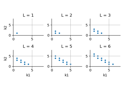
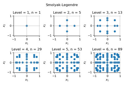
The Smolyak design of experiments (DOE) is based on a collection of marginal multidimensional elementary designs of experiments. Compared to the TensorProductExperiment, the Smolyak experiment has a significantly lower number of nodes [petras2003]. This implementation uses the combination technique ([gerstner1998] page 215). Smolyak quadrature involve weights which are negative ([sullivan2015] page 177). The size of the experiment is only known after the nodes and weights have been computed, that is, after the generateWithWeights() method is called.

Method

Let $\mathcal{X} \subset \mathbb{R}^{d_x}$ be the integration domain and let $g : \mathcal{X} \rightarrow \mathbb{R}^{d_y}$ be an integrable function. Let $f : \mathcal{X} \rightarrow \mathbb{R}$ be a probability density function. The Smolyak experiment produces an approximation of the integral:

$\int_{\mathcal{X}} g(\vect{x}) f(\vect{x}) d\vect{x} \approx \sum_{i = 1}^{s_t} w_i g\left(\vect{x}_i\right)$

where $s_t \in \mathbb{N}$ is the size of the Smolyak design of experiments, $w_1, ..., w_{s_t} \in \mathbb{R}$ are the weights and $\vect{x}_1, ..., \vect{x}_{s_t} \in \mathbb{R}^{d_x}$ are the nodes.

Let $\vect{k} = (k_1, ..., k_{d_x}) \in (\mathbb{N}^\star)^{d_x}$ be the multi-index where

$\mathbb{N}^\star = \{1, 2, ... \}$

is the set of natural numbers without zero. Consider the 1 and the infinity norms ([lemaitre2010] page 57, eq. 3.28):

$\|\vect{k}\|_1 = \sum_{i = 1}^{d_x} k_i \qquad \|\vect{k}\|_\infty = \max_{i = 1, ..., d_x} k_i.$

for any $\vect{k} \in (\mathbb{N}^\star)^{d_x}$ .

Let $\ell$ be an integer representing the level of the quadrature. Let $Q_{\ell}^{(1)}$ be a marginal quadrature of level $\ell$ . This marginal quadrature must have dimension 1 as is suggested by the exponent in the notation $Q_{\ell}^{(1)}$ . Depending on the level $\ell$ , we can compute the actual number of nodes depending on a particular choice of that number of nodes and depending on the quadrature rule. The tensor product quadrature is:

$T_\ell^{(d_x)} = Q_{\ell}^{(1)} \otimes ... \otimes Q_{\ell}^{(1)}.$

In the previous equation, the marginal quadratures are not necessarily of the same type. For example, if the dimension is equal to 2, the first marginal quadrature may be a Gaussian quadrature while the second one may be a random experiment, such as a Monte-Carlo design of experiment.

Let $Q_0^{(1)} = \emptyset$ be the empty quadrature. For any integer $k \in \mathbb{N}$ , let $\Delta_k^{(1)}$ be the difference quadrature defined by:

$\Delta_{k}^{(1)} = Q_{k}^{(1)} - Q_{k - 1}^{(1)}.$

Therefore, the quadrature formula $Q_\ell$ can be expressed depending on difference quadratures:

$Q_\ell^{(1)} = \sum_{k = 1}^\ell \Delta_k^{(1)}.$

for any $\ell \geq 1$ .

The following equation provides an equivalent equation for the tensor product quadrature ([lemaitre2010] page 57, eq. 3.30):

$T_\ell^{(d_x)} = \sum_{\|\vect{k}\|_\infty \leq \ell} \Delta_{k_1}^{(1)} \otimes \cdots \otimes \Delta_{k_{d_x}}^{(1)}.$

The significant part of the previous equation is the set of multi-indices $\|\vect{k}\|_\infty \leq \ell$ , which may be very large depending on the dimension of the problem.

One of the ways to reduce the size of this set is to consider the smaller set of multi-indices such that $\|\vect{k}\|_1 \leq \ell + {d_x} - 1$ . The sparse quadrature ([lemaitre2010] page 57, eq. 3.29, [gerstner1998] page 214) is introduced in the following definition.

The Smolyak sparse quadrature formula at level $\ell$ is:

$S_\ell^{(d_x)} = \sum_{\|\vect{k}\|_1 \leq \ell + d_x - 1} \Delta_{k_1}^{(1)} \otimes \cdots \otimes \Delta_{k_{d_x}}^{(1)}$

for any $\ell \geq 1$ .

As shown by the previous equation, for a given multi-index $\vect{k}$ the Smolyak quadrature requires to set the level of each marginal experiment to an integer which depends on the multi-index. This is done using the setLevel() method of the marginal quadrature.

The following formula expresses the multivariate quadrature in terms of combinations univariate quadratures, known as the combination technique. This method combines elementary tensorized quadratures, summing them depending on the binomial coefficient. The sparse quadrature formula at level $\ell$ is:

$S_\ell^{(d_x)} = \sum_{\ell \leq \|\vect{k}\|_1 \leq \ell + d_x - 1} (-1)^{\ell + d_x - \|\vect{k}\|_1 - 1} {d_x - 1 \choose \|\vect{k}\|_1 - \ell} Q_{k_1}^{(1)} \otimes \cdots \otimes Q_{k_{d_x}}^{(1)}$

for any $\ell \geq 1$ where the binomial coefficient is:

${n \choose m} = \frac{n!}{m! (n - m)!}$

for any integers $n \geq 0$ and $0 \leq m \leq n$ .

Merge duplicate nodes

The Smolyak quadrature requires to merge the potentially duplicated nodes of the elementary quadratures. To do so, a dictionary is used so that unique nodes only are kept. This algorithm is enabled by default, but it can be disabled with the SmolyakExperiment-MergeQuadrature boolean key of the ResourceMap. This can reduce the number of nodes, which may be particularly efficient when the marginal quadrature rule is nested such as, for example, with Fejér or Clenshaw-Curtis quadrature rule.

If two candidate nodes $\vect{x}_1, \vect{x}_2 \in \mathbb{R}^{d_x}$ , associated with the two weights $w_1, w_2 \in \mathbb{R}$ , are to be merged, then the merged node is

$\vect{x}_1' = \vect{x}_1$

and the merged weight is:

w_1' = w_1 + w_2.

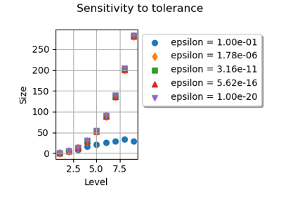
If, however, the elementary quadrature rules have nodes which are computed up to some rounding error, the merging algorithm may not detect that two nodes which are close to each other are, indeed, the same. This is why rounding errors must be taken into account. Let $\epsilon_r, \epsilon_a > 0$ be the relative and absolute tolerances. These parameters can be set using the ResourceMap keys SmolyakExperiment-MergeRelativeEpsilon and SmolyakExperiment-MergeAbsoluteEpsilon. The criterion is based on a mixed absolute and relative tolerance. Two candidate nodes $\vect{x}_1, \vect{x}_2 \in \mathbb{R}^{d_x}$ are close to each other and are to be merged if:

$|(x_1)_i - (y_1)_i| \leq \delta_i$

for $i = 1, ..., d_x$ , where $\delta_i$ is equal to:

$\delta_i = \epsilon_a + \epsilon_r \max\left(\left|(x_1)_i\right|, \left|(y_1)_i\right|\right).$

If the bounds of the input distribution are either very close to zero or very large, then the default settings may not work properly: in this case, please fine tune the parameters to match your needs.

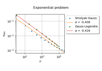
Accuracy

The following equation presents the absolute error of a sparse quadrature ([sullivan2015] page 177, eq. 9.10). Assume that $g \in \mathcal{C}^r([0, 1]^{d_x})$ and that we use a sparse quadrature with $n_\ell$ nodes at level $\ell$ . In this particular case, the probability density function $f$ is equal to 1. Therefore,

$\left|\int_{[0, 1]^{d_x}} g(\vect{x}) d\vect{x} - S_\ell(g)\right| = O \left(n_\ell^{-r} (\log(n_\ell))^{(d_x - 1)(r + 1)}\right).$

Examples

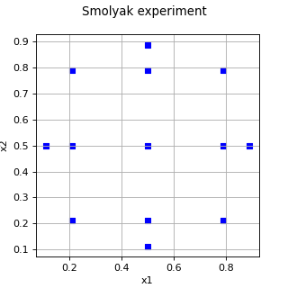
In the following example, we create Smolyak quadrature using two Gauss-Legendre marginal quadratures.

>>> import openturns as ot
>>> import openturns.experimental as otexp
>>> experiment1 = ot.GaussProductExperiment(ot.Uniform(0.0, 1.0))
>>> experiment2 = ot.GaussProductExperiment(ot.Uniform(0.0, 1.0))
>>> collection = [experiment1, experiment2]
>>> level = 3
>>> multivariate_experiment = otexp.SmolyakExperiment(collection, level)
>>> nodes, weights = multivariate_experiment.generateWithWeights()

Methods

`computeCombination`()	Compute the indices involved in the quadrature.
`generate`()	Generate points according to the type of the experiment.
`generateWithWeights`()	Generate points and their associated weight according to the type of the experiment.
`getClassName`()	Accessor to the object's name.
`getDistribution`()	Accessor to the distribution.
`getExperimentCollection`()	Get the marginals of the experiment.
`getId`()	Accessor to the object's id.
`getLevel`()	Get the level of the experiment.
`getName`()	Accessor to the object's name.
`getShadowedId`()	Accessor to the object's shadowed id.
`getSize`()	Accessor to the size of the generated sample.
`getVisibility`()	Accessor to the object's visibility state.
`hasName`()	Test if the object is named.
`hasUniformWeights`()	Ask whether the experiment has uniform weights.
`hasVisibleName`()	Test if the object has a distinguishable name.
`isRandom`()	Accessor to the randomness of quadrature.
`setDistribution`(distribution)	Accessor to the distribution.
`setExperimentCollection`(coll)	Set the marginals of the experiment.
`setLevel`(level)	Set the level of the experiment.
`setName`(name)	Accessor to the object's name.
`setShadowedId`(id)	Accessor to the object's shadowed id.
`setSize`(size)	Accessor to the size of the generated sample.
`setVisibility`(visible)	Accessor to the object's visibility state.

__init__(*args)¶

computeCombination()¶

Compute the indices involved in the quadrature.

Returns:

indicesCollectionlist of IndicesCollection: List of the multi-indices involved in Smolyak’s quadrature.

generate()¶

Generate points according to the type of the experiment.

Returns:

sampleSample: Points $(\Xi_i)_{i \in I}$ which constitute the design of experiments with $card I = size$ . The sampling method is defined by the nature of the weighted experiment.

Examples

>>> import openturns as ot
>>> ot.RandomGenerator.SetSeed(0)
>>> myExperiment = ot.MonteCarloExperiment(ot.Normal(2), 5)
>>> sample = myExperiment.generate()
>>> print(sample)
    [ X0        X1        ]
0 : [  0.608202 -1.26617  ]
1 : [ -0.438266  1.20548  ]
2 : [ -2.18139   0.350042 ]
3 : [ -0.355007  1.43725  ]
4 : [  0.810668  0.793156 ]

generateWithWeights()¶

Generate points and their associated weight according to the type of the experiment.

Returns:

sampleSample: The points which constitute the design of experiments. The sampling method is defined by the nature of the experiment.
weightsPoint of size $cardI$: Weights $(\omega_i)_{i \in I}$ associated with the points. By default, all the weights are equal to $1/cardI$ .

Examples

>>> import openturns as ot
>>> ot.RandomGenerator.SetSeed(0)
>>> myExperiment = ot.MonteCarloExperiment(ot.Normal(2), 5)
>>> sample, weights = myExperiment.generateWithWeights()
>>> print(sample)
    [ X0        X1        ]
0 : [  0.608202 -1.26617  ]
1 : [ -0.438266  1.20548  ]
2 : [ -2.18139   0.350042 ]
3 : [ -0.355007  1.43725  ]
4 : [  0.810668  0.793156 ]
>>> print(weights)
[0.2,0.2,0.2,0.2,0.2]

getClassName()¶

Accessor to the object’s name.

Returns:

class_namestr: The object class name (object.__class__.__name__).

getDistribution()¶

Accessor to the distribution.

Returns:

distributionDistribution: Distribution used to generate the set of input data.

getExperimentCollection()¶

Get the marginals of the experiment.

Returns:

experimentslist of WeightedExperiment: List of the marginals of the experiment.

getId()¶

Accessor to the object’s id.

Returns:

idint: Internal unique identifier.

getLevel()¶

Get the level of the experiment.

Returns:

levelint: Level value $\ell \geq 1$ .

getName()¶

Accessor to the object’s name.

Returns:

namestr: The name of the object.

getShadowedId()¶

Accessor to the object’s shadowed id.

Returns:

idint: Internal unique identifier.

getSize()¶

Accessor to the size of the generated sample.

Returns:

sizepositive int: Number $cardI$ of points constituting the design of experiments.

getVisibility()¶

Accessor to the object’s visibility state.

Returns:

visiblebool: Visibility flag.

hasName()¶

Test if the object is named.

Returns:

hasNamebool: True if the name is not empty.

hasUniformWeights()¶

Ask whether the experiment has uniform weights.

Returns:

hasUniformWeightsbool: Whether the experiment has uniform weights.

hasVisibleName()¶

Test if the object has a distinguishable name.

Returns:

hasVisibleNamebool: True if the name is not empty and not the default one.

isRandom()¶

Accessor to the randomness of quadrature.

Parameters:

isRandombool: Is true if the design of experiments is random. Otherwise, the design of experiment is assumed to be deterministic.

setDistribution(distribution)¶

Accessor to the distribution.

Parameters:

distributionDistribution: Distribution used to generate the set of input data.

setExperimentCollection(coll)¶

Set the marginals of the experiment.

Parameters:

experimentslist of WeightedExperiment: List of the marginals of the experiment.

setLevel(level)¶

Set the level of the experiment.

Parameters:

levelint: Level value $\ell \geq 1$ .

setName(name)¶

Accessor to the object’s name.

Parameters:

namestr: The name of the object.

setShadowedId(id)¶

Accessor to the object’s shadowed id.

Parameters:

idint: Internal unique identifier.

setSize(size)¶

Accessor to the size of the generated sample.

Parameters:

sizepositive int: Number $cardI$ of points constituting the design of experiments.

setVisibility(visible)¶

Accessor to the object’s visibility state.

Parameters:

visiblebool: Visibility flag.

Examples using the class¶

Plot Smolyak multi-indices

Plot the Smolyak quadrature

Merge nodes in Smolyak quadrature

Use the Smolyak quadrature

OpenTURNS

An Open source initiative for the Treatment of Uncertainties, Risks'N Statistics

Table of Contents

Previous topic

Next topic

This Page

SmolyakExperiment¶

Examples using the class¶