RP55 analysis and 2D graphics

The objective of this example is to present problem 55 of the BBRC. We also present graphic elements for the visualization of the limit state surface in 2 dimensions.

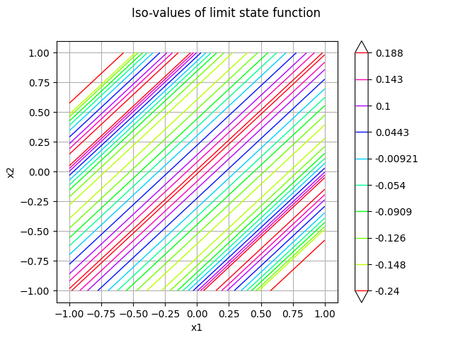
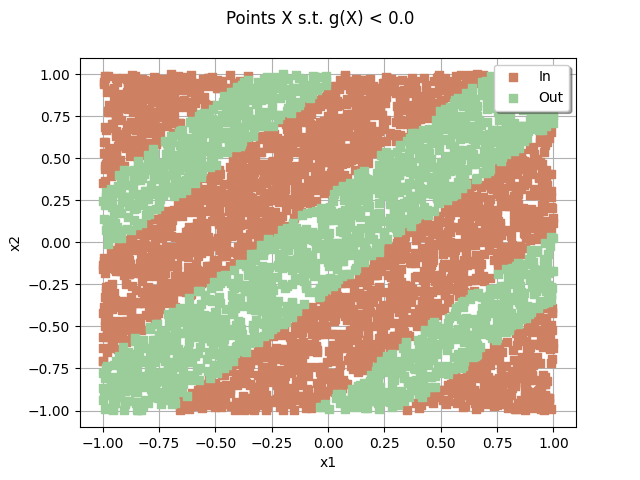
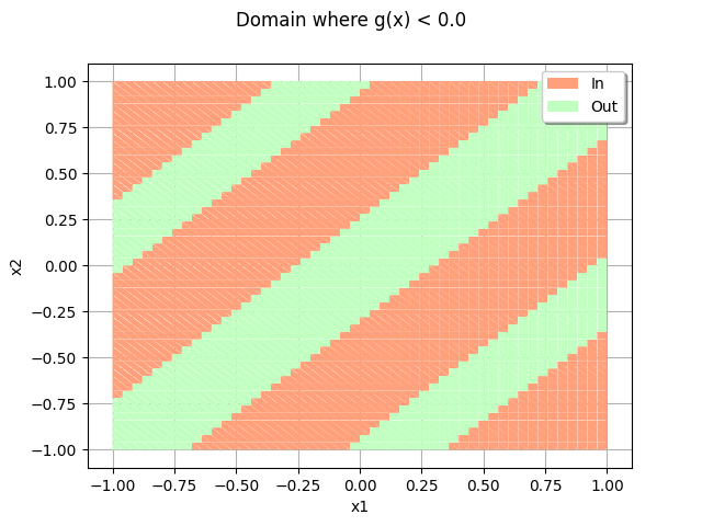
The dimension is equal to 2 and the probability is close to $10^{-2}$. This makes this problem relatively easy to solve. The distribution is uniform in the square $[-1,1]^2$. The failure domain is made of 5 diagonal bands. Capturing these bands is relatively easy and a Monte-Carlo simulation perform well in this case. The FORM method cannot perform correctly, since the failure domain cannot be linearized in the gaussian space. Hence, the SORM or FORM-IS methods do not perform satisfactorily.

import openturns as ot
import otbenchmark as otb
import openturns.viewer as otv

Disable warnings

ot.Log.Show(ot.Log.NONE)

problem = otb.ReliabilityProblem55()
print(problem)

name = RP55
event = class=ThresholdEventImplementation antecedent=class=CompositeRandomVector function=class=Function name=Unnamed implementation=class=FunctionImplementation name=Unnamed description=[x1,x2,gsys] evaluationImplementation=class=SymbolicEvaluation name=Unnamed inputVariablesNames=[x1,x2] outputVariablesNames=[gsys] formulas=[var g1 := 0.2 + 0.6 * (x1 - x2)^4 - (x1 - x2) / sqrt(2);var g2 := 0.2 + 0.6 * (x1 - x2)^4 + (x1 - x2) / sqrt(2);var g3 := (x1 - x2) + 5 / sqrt(2) - 2.2;var g4 := (x2 - x1) + 5 / sqrt(2) - 2.2;gsys := min(g1, g2, g3, g4)] gradientImplementation=class=SymbolicGradient name=Unnamed evaluation=class=SymbolicEvaluation name=Unnamed inputVariablesNames=[x1,x2] outputVariablesNames=[gsys] formulas=[var g1 := 0.2 + 0.6 * (x1 - x2)^4 - (x1 - x2) / sqrt(2);var g2 := 0.2 + 0.6 * (x1 - x2)^4 + (x1 - x2) / sqrt(2);var g3 := (x1 - x2) + 5 / sqrt(2) - 2.2;var g4 := (x2 - x1) + 5 / sqrt(2) - 2.2;gsys := min(g1, g2, g3, g4)] hessianImplementation=class=SymbolicHessian name=Unnamed evaluation=class=SymbolicEvaluation name=Unnamed inputVariablesNames=[x1,x2] outputVariablesNames=[gsys] formulas=[var g1 := 0.2 + 0.6 * (x1 - x2)^4 - (x1 - x2) / sqrt(2);var g2 := 0.2 + 0.6 * (x1 - x2)^4 + (x1 - x2) / sqrt(2);var g3 := (x1 - x2) + 5 / sqrt(2) - 2.2;var g4 := (x2 - x1) + 5 / sqrt(2) - 2.2;gsys := min(g1, g2, g3, g4)] antecedent=class=UsualRandomVector distribution=class=JointDistribution name=JointDistribution dimension=2 copula=class=IndependentCopula name=IndependentCopula dimension=2 marginal[0]=class=Uniform name=Uniform dimension=1 a=-1 b=1 marginal[1]=class=Uniform name=Uniform dimension=1 a=-1 b=1 operator=class=Less name=Unnamed threshold=0
probability = 0.5600144282863704

event = problem.getEvent()
g = event.getFunction()

problem.getProbability()

0.5600144282863704

Compute the bounds of the domain

inputVector = event.getAntecedent()
distribution = inputVector.getDistribution()
X1 = distribution.getMarginal(0)
X2 = distribution.getMarginal(1)
alphaMin = 0.00001
alphaMax = 1 - alphaMin
lowerBound = ot.Point(
    [X1.computeQuantile(alphaMin)[0], X2.computeQuantile(alphaMin)[0]]
)
upperBound = ot.Point(
    [X1.computeQuantile(alphaMax)[0], X2.computeQuantile(alphaMax)[0]]
)

nbPoints = [100, 100]
figure = g.draw(lowerBound, upperBound, nbPoints)
figure.setTitle("Iso-values of limit state function")
_ = otv.View(figure)

Plot the iso-values of the distribution

_ = otv.View(distribution.drawPDF())

sampleSize = 5000
sampleInput = inputVector.getSample(sampleSize)
sampleOutput = g(sampleInput)
drawEvent = otb.DrawEvent(event)

cloud = drawEvent.drawSampleCrossCut(sampleSize)
_ = otv.View(cloud)

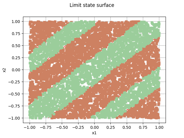
Draw the limit state surface

bounds = ot.Interval(lowerBound, upperBound)
bounds

class=Interval name=Unnamed dimension=2 lower bound=class=Point name=Unnamed dimension=2 values=[-0.99998,-0.99998] upper bound=class=Point name=Unnamed dimension=2 values=[0.99998,0.99998] finite lower bound=[1,1] finite upper bound=[1,1]

graph = drawEvent.drawLimitStateCrossCut(bounds)
graph.add(cloud)
_ = otv.View(graph)

domain = drawEvent.fillEventCrossCut(bounds)
_ = otv.View(domain)

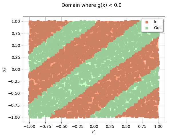
domain.add(cloud)
_ = otv.View(domain)

Perform Monte-Carlo simulation

algoProb = ot.ProbabilitySimulationAlgorithm(event)
algoProb.setMaximumOuterSampling(1000)
algoProb.setMaximumCoefficientOfVariation(0.01)
algoProb.run()

resultAlgo = algoProb.getResult()
neval = g.getEvaluationCallsNumber()
print("Number of function calls = %d" % (neval))
pf = resultAlgo.getProbabilityEstimate()
print("Failure Probability = %.4f" % (pf))
level = 0.95
c95 = resultAlgo.getConfidenceLength(level)
pmin = pf - 0.5 * c95
pmax = pf + 0.5 * c95
print("%.1f %% confidence interval :[%.4f,%.4f] " % (level * 100, pmin, pmax))

Number of function calls = 43704
Failure Probability = 0.5620
95.0 % confidence interval :[0.5312,0.5928]

With FORM-IS

maximumEvaluationNumber = 1000
maximumAbsoluteError = 1.0e-3
maximumRelativeError = 1.0e-3
maximumResidualError = 1.0e-3
maximumConstraintError = 1.0e-3
nearestPointAlgorithm = ot.AbdoRackwitz()
nearestPointAlgorithm.setMaximumCallsNumber(maximumEvaluationNumber)
nearestPointAlgorithm.setMaximumAbsoluteError(maximumAbsoluteError)
nearestPointAlgorithm.setMaximumRelativeError(maximumRelativeError)
nearestPointAlgorithm.setMaximumResidualError(maximumResidualError)
nearestPointAlgorithm.setMaximumConstraintError(maximumConstraintError)

metaAlgorithm = otb.ReliabilityBenchmarkMetaAlgorithm(problem)
benchmarkResult = metaAlgorithm.runFORMImportanceSampling(
    nearestPointAlgorithm, maximumOuterSampling=10 ** 5, coefficientOfVariation=0.0
)

print(benchmarkResult.summary())

computedProbability = 0.0
exactProbability = 0.5600144282863704
absoluteError = 0.5600144282863704
numberOfCorrectDigits = 0.0
numberOfFunctionEvaluations = 1006
numberOfDigitsPerEvaluation = 0.0

With Quasi-Monte-Carlo

sequence = ot.SobolSequence()
experiment = ot.LowDiscrepancyExperiment(sequence, 1)
experiment.setRandomize(False)

algo = ot.ProbabilitySimulationAlgorithm(event, experiment)
algo.setMaximumOuterSampling(10 ** 3)
algo.setMaximumCoefficientOfVariation(0.0)
algo.setBlockSize(10 ** 3)
algo.run()

result = algo.getResult()
probability = result.getProbabilityEstimate()
print("Pf=", probability)

Pf= 0.5593869999999994

otv.View.ShowAll()