Using the FORM - SORM algorithms on a nonlinear function

In this example, we estimate a failure probability with the FORM and SORM algorithms on the oscillator example. This test-case is highly non linear with a significant curvature near the design point.

Model definition

from openturns.usecases import oscillator
import openturns as ot
from matplotlib import pylab as plt
import numpy as np

ot.Log.Show(ot.Log.NONE)
ot.RandomGenerator.SetSeed(1)

We load the model from the usecases module:

osc = oscillator.Oscillator()

We use the input parameters distribution from the data class:

distribution = osc.distribution

We define the model:

model = osc.model

We create the event whose probability we want to estimate.

vect = ot.RandomVector(distribution)
G = ot.CompositeRandomVector(model, vect)
event = ot.ThresholdEvent(G, ot.Less(), 0.0)
event.setName("failure")

Cross cuts in the physical space

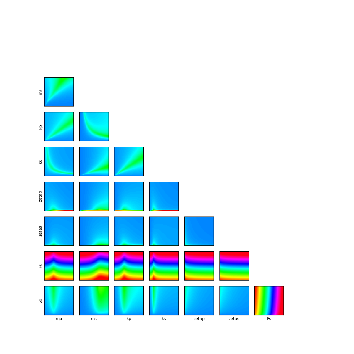
Let’s have a look on 2D cross cuts of the limit state function. For each 2D cross cut, the other variables are fixed to the input distribution mean values. This graph allows one to have a first idea of the variations of the function in pairs of dimensions. The colors of each contour plot are comparable. The number of contour levels are related to the amount of variation of the function in the corresponding coordinates.

fig = plt.figure(figsize=(12, 12))
lowerBound = [1e-5] * 8
upperBound = distribution.getRange().getUpperBound()

# Definition of number of meshes in x and y axes for the 2D cross cut plots
nX = 50
nY = 50
for i in range(distribution.getDimension()):
    for j in range(i):
        crossCutIndices = []
        crossCutReferencePoint = []
        for k in range(distribution.getDimension()):
            if k != i and k != j:
                crossCutIndices.append(k)
                # Definition of the reference point
                crossCutReferencePoint.append(distribution.getMean()[k])
        # Definition of 2D cross cut function
        crossCutFunction = ot.ParametricFunction(
            model, crossCutIndices, crossCutReferencePoint
        )
        crossCutLowerBound = [lowerBound[j], lowerBound[i]]
        crossCutUpperBound = [upperBound[j], upperBound[i]]
        # Definition of the mesh
        inputData = ot.Box([nX, nY]).generate()
        inputData *= ot.Point(crossCutUpperBound) - ot.Point(crossCutLowerBound)
        inputData += ot.Point(crossCutLowerBound)
        meshX = np.array(inputData)[:, 0].reshape(nX + 2, nY + 2)
        meshY = np.array(inputData)[:, 1].reshape(nX + 2, nY + 2)
        data = crossCutFunction(inputData)
        meshZ = np.array(data).reshape(nX + 2, nY + 2)
        levels = [(150 + 3 * i) for i in range(101)]

        # Creation of the contour
        index = 1 + i * distribution.getDimension() + j

        ax = fig.add_subplot(
            distribution.getDimension(), distribution.getDimension(), index
        )
        ax.pcolormesh(meshX, meshY, meshZ, cmap="hsv", vmin=-5, vmax=50, shading="auto")
        ax.set_xticks([])
        ax.set_yticks([])
        # Creation of axes title
        if j == 0:
            ax.set_ylabel(distribution.getDescription()[i])
        if i == 7:
            ax.set_xlabel(distribution.getDescription()[j])

Computation of reference probability with Monte-Carlo simulation

The target probability is supposed to be extremely low (). Indeed, when performing Monte-Carlo simulation with a simulation budget of 100000 points, no sample are in the failure state, that induces a probability estimate of zero.

experiment = ot.MonteCarloExperiment()
algo = ot.ProbabilitySimulationAlgorithm(event, experiment)
algo.setMaximumOuterSampling(int(1e5))
algo.run()

result = algo.getResult()
probability = result.getProbabilityEstimate()
print("Failure probability = ", probability)

Failure probability =  0.0

To get an accurate estimate of this probability, a billion of simulations are necessary.

FORM Analysis

To get a first idea of the failure probability with reduced simulation budget, one can use the First Order Reliability Method (FORM).

Define a solver:

optimAlgo = ot.Cobyla()
optimAlgo.setMaximumCallsNumber(1000)
optimAlgo.setMaximumAbsoluteError(1.0e-3)
optimAlgo.setMaximumRelativeError(1.0e-3)
optimAlgo.setMaximumResidualError(1.0e-3)
optimAlgo.setMaximumConstraintError(1.0e-3)

Run FORM initialized at the mean of the distribution:

algo = ot.FORM(optimAlgo, event, distribution.getMean())
algo.run()
result = algo.getResult()

Probability of failure:

print("FORM estimate of the probability of failure: ", result.getEventProbability())

FORM estimate of the probability of failure:  3.891496415542106e-06

Design point in the standard space:

designPointStandardSpace = result.getStandardSpaceDesignPoint()
print("Design point in standard space : ", designPointStandardSpace)

Design point in standard space :  [0.292325,1.2089,1.28593,-0.286932,-2.85666,-1.8419,-2.03238,1.01191]

Design point in the physical space:

print("Design point in physical space : ", result.getPhysicalSpaceDesignPoint())

Design point in physical space :  [1.53672,0.0112256,1.26498,0.00926413,0.0154449,0.00749384,22.3422,110.072]

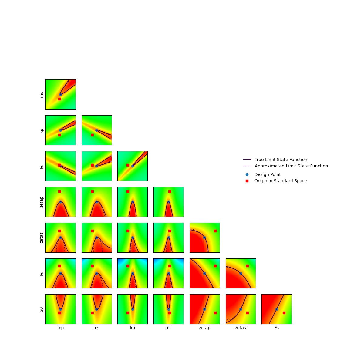
For this test case, in order to validate the results obtained by FORM, we can plot the cross cuts in the standard space near the design point found by FORM.

distributionStandard = ot.Normal(distribution.getDimension())
inverseIsoProbabilistic = distribution.getInverseIsoProbabilisticTransformation()
standardSpaceLimitState = ot.ComposedFunction(model, inverseIsoProbabilistic)
standardSpaceLimitStateFunction = ot.PythonFunction(8, 1, standardSpaceLimitState)

fig = plt.figure(figsize=(12, 12))
lowerBound = [-4] * 8
upperBound = [4] * 8

# sphinx_gallery_thumbnail_number = 2

# Definition of number of meshes in x and y axes for the 2D cross cut plots
nX = 50
nY = 50
my_labels = {
    "MPP": "Design Point",
    "O": "Origin in Standard Space",
    "TLSF": "True Limit State Function",
    "ALSF": "Approximated Limit State Function",
}
for i in range(distribution.getDimension()):
    for j in range(i):
        crossCutIndices = []
        crossCutReferencePoint = []
        for k in range(distribution.getDimension()):
            if k != i and k != j:
                crossCutIndices.append(k)
                # Definition of the reference point
                crossCutReferencePoint.append(designPointStandardSpace[k])
        # Definition of 2D cross cut function
        crossCutFunction = ot.ParametricFunction(
            standardSpaceLimitStateFunction, crossCutIndices, crossCutReferencePoint
        )

        crossCutLowerBound = [
            lowerBound[j] + designPointStandardSpace[j],
            lowerBound[i] + designPointStandardSpace[i],
        ]
        crossCutUpperBound = [
            upperBound[j] + designPointStandardSpace[j],
            upperBound[i] + designPointStandardSpace[i],
        ]
        # Definition of the mesh
        inputData = ot.Box([nX, nY]).generate()
        inputData *= ot.Point(crossCutUpperBound) - ot.Point(crossCutLowerBound)
        inputData += ot.Point(crossCutLowerBound)
        meshX = np.array(inputData)[:, 0].reshape(nX + 2, nY + 2)
        meshY = np.array(inputData)[:, 1].reshape(nX + 2, nY + 2)
        data = crossCutFunction(inputData)
        meshZ = np.array(data).reshape(nX + 2, nY + 2)
        levels = [(150 + 3 * i) for i in range(101)]

        # Creation of the contour
        index = 1 + i * distribution.getDimension() + j

        ax = fig.add_subplot(
            distribution.getDimension(), distribution.getDimension(), index
        )

        graph = ot.Graph()

        ax.pcolormesh(meshX, meshY, meshZ, cmap="hsv", vmin=-5, vmax=50, shading="auto")

        cs0 = ax.plot(
            designPointStandardSpace[j],
            designPointStandardSpace[i],
            "o",
            label=my_labels["MPP"],
        )
        cs1 = ax.plot(0.0, 0.0, "rs", label=my_labels["O"])
        cs2 = ax.contour(meshX, meshY, meshZ, [0.0])

        ax.set_xticks([])
        ax.set_yticks([])

        u0 = [designPointStandardSpace[j], designPointStandardSpace[i]]
        algo = ot.LinearTaylor(u0, crossCutFunction)
        algo.run()
        responseSurface = algo.getMetaModel()
        data2 = responseSurface(inputData)
        meshZ2 = np.array(data2).reshape(nX + 2, nY + 2)

        cs3 = ax.contour(meshX, meshY, meshZ2, [0.0], linestyles="dotted")

        # Creation of axes title
        if j == 0:
            ax.set_ylabel(distribution.getDescription()[i])
        if i == 7:
            ax.set_xlabel(distribution.getDescription()[j])

        if i == 1 and j == 0:
            cs2.collections[0].set_label(my_labels["TLSF"])
            h2, l2 = cs2.legend_elements()
            cs3.collections[0].set_label(my_labels["ALSF"])
            h3, l3 = cs3.legend_elements()
            lg = ax.legend(
                [h2[0], h3[0]],
                [my_labels["TLSF"], my_labels["ALSF"]],
                frameon=False,
                loc="upper center",
                bbox_to_anchor=(8, -1.5),
            )
        elif i == 2 and j == 0:
            lg1 = ax.legend(
                frameon=False, loc="upper center", bbox_to_anchor=(7.65, -0.8)
            )

As it can be seen, the curvature of the limit state function near the design point is significant. In that way, FORM provides poor estimate since it linearly approximates the limit state function. Thus, SORM can be used in order to refine this probability estimation by approximating the limit state function with a quadratic model.

SORM Analysis

Run SORM initialized at the mean of the distribution:

algoSORM = ot.SORM(ot.Cobyla(), event, distribution.getMean())
algoSORM.run()

Analysis of SORM results:

resultSORM = algoSORM.getResult()
print(
    "Probability estimate with SORM (Breitung correction) =",
    resultSORM.getEventProbabilityBreitung(),
)

print(
    "Probability estimate with SORM (Hohenbichler correction) =",
    resultSORM.getEventProbabilityHohenbichler(),
)

optim_res = resultSORM.getOptimizationResult()
print("Simulation budget:", optim_res.getEvaluationNumber())

Probability estimate with SORM (Breitung correction) = 3.8119422417743107e-07
Probability estimate with SORM (Hohenbichler correction) = 3.6841954700676055e-07
Simulation budget: 783

One can see that the probability estimate has been decreased by a factor 10 compared to the FORM estimate. This probability is quite close to the reference probability and obtained with less than 1000 evaluations of the model.

In order to visualize the SORM limit state approximation, we can draw cross cuts of SORM oscultating parabola using second order Taylor approximation.

fig = plt.figure(figsize=(12, 12))
lowerBound = [-4] * 8
upperBound = [4] * 8

# Definition of number of meshes in x and y axes for the 2D cross cut plots
nX = 50
nY = 50

my_labels = {
    "MPP": "Design Point",
    "O": "Origin in Standard Space",
    "TLSF": "True Limit State Function",
    "ALSF": "Approximated Limit State Function",
}

for i in range(distribution.getDimension()):
    for j in range(i):
        crossCutIndices = []
        crossCutReferencePoint = []
        for k in range(distribution.getDimension()):
            if k != i and k != j:
                crossCutIndices.append(k)
                # Definition of the reference point
                crossCutReferencePoint.append(designPointStandardSpace[k])
        # Definition of 2D cross cut function
        crossCutFunction = ot.ParametricFunction(
            standardSpaceLimitStateFunction, crossCutIndices, crossCutReferencePoint
        )

        crossCutLowerBound = [
            lowerBound[j] + designPointStandardSpace[j],
            lowerBound[i] + designPointStandardSpace[i],
        ]
        crossCutUpperBound = [
            upperBound[j] + designPointStandardSpace[j],
            upperBound[i] + designPointStandardSpace[i],
        ]
        # Definition of the mesh
        inputData = ot.Box([nX, nY]).generate()
        inputData *= ot.Point(crossCutUpperBound) - ot.Point(crossCutLowerBound)
        inputData += ot.Point(crossCutLowerBound)
        meshX = np.array(inputData)[:, 0].reshape(nX + 2, nY + 2)
        meshY = np.array(inputData)[:, 1].reshape(nX + 2, nY + 2)
        data = crossCutFunction(inputData)
        meshZ = np.array(data).reshape(nX + 2, nY + 2)
        levels = [(150 + 3 * i) for i in range(101)]

        # Creation of the contour
        index = 1 + i * distribution.getDimension() + j

        ax = fig.add_subplot(
            distribution.getDimension(), distribution.getDimension(), index
        )

        graph = ot.Graph()
        ax.pcolormesh(meshX, meshY, meshZ, cmap="hsv", vmin=-5, vmax=50, shading="auto")
        cs0 = ax.plot(
            designPointStandardSpace[j],
            designPointStandardSpace[i],
            "o",
            label=my_labels["MPP"],
        )
        cs1 = ax.plot(0.0, 0.0, "rs", label=my_labels["O"])
        cs2 = ax.contour(meshX, meshY, meshZ, [0.0])
        ax.set_xticks([])
        ax.set_yticks([])

        u0 = [designPointStandardSpace[j], designPointStandardSpace[i]]
        algo = ot.QuadraticTaylor(u0, crossCutFunction)
        algo.run()
        responseSurface = algo.getMetaModel()
        data2 = responseSurface(inputData)
        meshZ2 = np.array(data2).reshape(nX + 2, nY + 2)
        cs3 = ax.contour(meshX, meshY, meshZ2, [0.0], linestyles="dotted")

        # Creation of axes title
        if j == 0:
            ax.set_ylabel(distribution.getDescription()[i])
        if i == 7:
            ax.set_xlabel(distribution.getDescription()[j])

        if i == 1 and j == 0:
            cs2.collections[0].set_label(my_labels["TLSF"])
            h2, l2 = cs2.legend_elements()
            cs3.collections[0].set_label(my_labels["ALSF"])
            h3, l3 = cs3.legend_elements()
            lg = ax.legend(
                [h2[0], h3[0]],
                [my_labels["TLSF"], my_labels["ALSF"]],
                frameon=False,
                loc="upper center",
                bbox_to_anchor=(8, -1.5),
            )
        elif i == 2 and j == 0:
            lg1 = ax.legend(
                frameon=False, loc="upper center", bbox_to_anchor=(7.65, -0.8)
            )

We can see that this approximation is very appropriate, explaining the accuracy of the obtained results.

Estimation with post analytical Importance Sampling

Different algorithms exist for the reliability analysis by Importance Sampling. One way is to perform post analytical Importance Sampling by defining the auxiliary density centered at the design point found by FORM.

postAnalyticalIS = ot.PostAnalyticalImportanceSampling(result)
postAnalyticalIS.setMaximumCoefficientOfVariation(0.05)
postAnalyticalIS.run()
resultPostAnalyticalIS = postAnalyticalIS.getResult()
print(
    "Probability of failure with post analytical IS = ",
    resultPostAnalyticalIS.getProbabilityEstimate(),
)

Probability of failure with post analytical IS =  3.948977006146584e-07

We can see that this post-treatment of FORM result allows one to greatly improve the quality of the probability estimation.