Note
Go to the end to download the full example code.
Non parametric Adaptive Importance Sampling (NAIS)
The objective is to evaluate a probability from the Non parametric Adaptive Importance Sampling (NAIS) technique.
We consider the four-branch function defined by:
and the input random vector which follows the standard 2-dimensional Normal distribution:
We want to evaluate the probability:
First, import the python modules:
import openturns as ot
from openturns.viewer import View
import math
Create the probabilistic model  
Create the input random vector :
X = ot.RandomVector(ot.Normal(2))
Create the function from a
PythonFunction:
def fourBranch(x):
    x1 = x[0]
    x2 = x[1]

    g1 = 5 + 0.1 * (x1 - x2) ** 2 - (x1 + x2) / math.sqrt(2)
    g2 = 5 + 0.1 * (x1 - x2) ** 2 + (x1 + x2) / math.sqrt(2)
    g3 = (x1 - x2) + 9 / math.sqrt(2)
    g4 = (x2 - x1) + 9 / math.sqrt(2)

    return [min((g1, g2, g3, g4))]


g = ot.PythonFunction(2, 1, fourBranch)
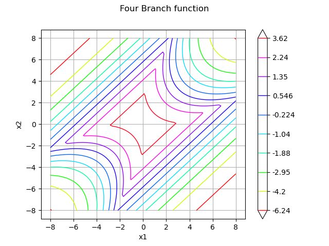
Draw the function to help to understand the shape of the limit state function:
graph = ot.Graph("Four Branch function", "x1", "x2", True, "upper right")
drawfunction = g.draw([-8] * 2, [8] * 2, [100] * 2)
graph.add(drawfunction)
view = View(graph)

In order to be able to get the NAIS samples used in the algorithm, it is necessary to transform the PythonFunction into a MemoizeFunction:
g = ot.MemoizeFunction(g)
Create the output random vector :
Y = ot.CompositeRandomVector(g, X)
Create the event  
threshold = 0.0
myEvent = ot.ThresholdEvent(Y, ot.Less(), threshold)
Evaluate the probability with the NAIS technique
quantileLevel = 0.1
algo = ot.NAIS(myEvent, quantileLevel)
In order to get all the inputs and outputs that realize the event, you have to mention it now:
algo.setKeepSample(True)
Now you can run the algorithm.
algo.run()
result = algo.getResult()
proba = result.getProbabilityEstimate()
print("Proba NAIS = ", proba)
print("Current coefficient of variation = ", result.getCoefficientOfVariation())
Proba NAIS =  6.783040767375951e-06
Current coefficient of variation =  0.09906313104733465
The length of the confidence interval of level is:
length95 = result.getConfidenceLength()
print("Confidence length (0.95) = ", result.getConfidenceLength())
Confidence length (0.95) = 2.6339926841138084e-06
which enables to build the confidence interval:
print(
    "Confidence interval (0.95) = [",
    proba - length95 / 2,
    ", ",
    proba + length95 / 2,
    "]",
)
Confidence interval (0.95) = [ 5.466044425319046e-06 , 8.100037109432855e-06 ]
You can also get the successive thresholds used by the algorithm:
levels = algo.getThresholdPerStep()
print("Levels of g = ", levels)
Levels of g = [3.40173,2.03082,0.448448,0]
Draw the NAIS samples used by the algorithm
You can get the number of steps with:
Ns = algo.getStepsNumber()
print("Number of steps= ", Ns)
Number of steps= 4
Get all the inputs where was evaluated at each step
list_subSamples = list()
for step in range(Ns):
    list_subSamples.append(algo.getInputSample(step))
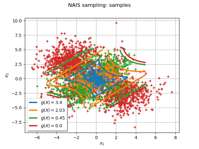
The following graph draws each NAIS sample and the frontier where
is the threshold at the step
:
graph = ot.Graph()
graph.setAxes(True)
graph.setGrid(True)
graph.setTitle("NAIS sampling: samples")
graph.setXTitle(r"$x_1$")
graph.setYTitle(r"$x_2$")
graph.setLegendPosition("lower left")
Add all the NAIS samples:
for i in range(Ns):
    cloud = ot.Cloud(list_subSamples[i])
    # cloud.setPointStyle("dot")
    graph.add(cloud)
col = graph.getColors()
Add the frontiers where
is the threshold at the step
:
gIsoLines = g.draw([-5] * 2, [5] * 2, [128] * 2)
dr = gIsoLines.getDrawable(0)
for i, lv in enumerate(levels):
    dr.setLevels([lv])
    dr.setLineStyle("solid")
    dr.setLegend(r"$g(X) = $" + str(round(lv, 2)))
    dr.setLineWidth(3)
    dr.setColor(col[i])
    graph.add(dr)
_ = View(graph)

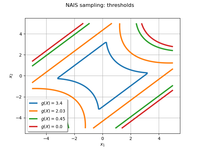
Draw the frontiers only
The following graph enables to understand the progression of the algorithm:
graph = ot.Graph()
graph.setAxes(True)
graph.setGrid(True)
dr = gIsoLines.getDrawable(0)
for i, lv in enumerate(levels):
    dr.setLevels([lv])
    dr.setLineStyle("solid")
    dr.setLegend(r"$g(X) = $" + str(round(lv, 2)))
    dr.setLineWidth(3)
    graph.add(dr)

graph.setColors(col)
graph.setLegendPosition("lower left")
graph.setTitle("NAIS sampling: thresholds")
graph.setXTitle(r"$x_1$")
graph.setYTitle(r"$x_2$")

_ = View(graph)

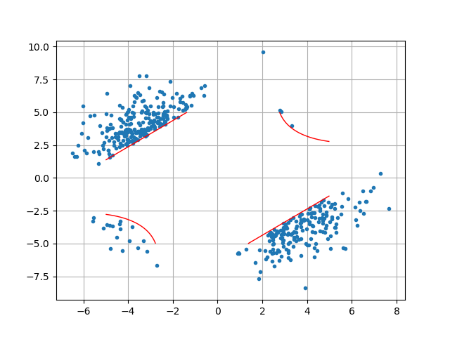
Get all the input and output points that realized the event
The following lines are possible only if you have mentioned that you wanted to keep samples with the method algo.setKeepSample(True)
select = ot.NAIS.EVENT1  # points that realize the event
step = Ns - 1  # get the working sample from last iteration
inputEventSample = algo.getInputSample(step, select)
outputEventSample = algo.getOutputSample(step, select)
print("Number of event realizations = ", inputEventSample.getSize())
Number of event realizations = 441
Draw them! They are all in the event space.
graph = ot.Graph()
graph.setAxes(True)
graph.setGrid(True)
cloud = ot.Cloud(inputEventSample)
cloud.setPointStyle("bullet")
graph.add(cloud)
gIsoLines = g.draw([-5] * 2, [5] * 2, [1000] * 2)
dr = gIsoLines.getDrawable(0)
dr.setLevels([0.0])
dr.setColor("red")
graph.add(dr)
_ = View(graph)

View.ShowAll()

Total running time of the script: (0 minutes 2.842 seconds)
 OpenTURNS