The Kolmogorov-Smirnov goodness of fit test for continuous data
The Kolmogorov-Smirnov test is a statistical test of whether a given sample of data is drawn from a given probability distribution which is of dimension 1 and continuous.
Let be a sample of dimension 1 drawn from the (unknown) cumulative distribution function
.
We want to test whether the sample is drawn from the cumulative distribution function
.
This test involves the calculation of the test statistic which is the weighted maximum
distance between the empirical cumulative distribution function
and
.
Letting
be independent random variables respectively distributed according to
, then
is defined by:
for all . The test statistic is defined by:
The empirical value of the test statistic is denoted by , using the realization of
on the sample:
Under the null hypothesis , the distribution of
the test statistic
is
known: algorithms are available to compute the distribution of
both for
large (asymptotic distribution: this is the Kolmogorov distribution) or for
small (exact distribution). Then we can use that
distribution to apply the test as follows.
We fix a risk
(error type I) and we evaluate the associated critical
value
which is the quantile of order
of
.
Then a decision is made, either by comparing the test statistic to the theoretical
threshold
(or equivalently
by evaluating the p-value of the sample defined as
and by comparing
it to
):
if
(or equivalently
), then we reject
,
if
(or equivalently
), then
is considered acceptable.
It is assumed that the parameters of the continuous distribution which is tested have not been inferred from the sample. If this is the case, we have to use the Lilliefors test rather than the Kolmogorov test.
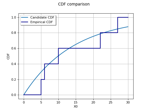
The figure below illustrates the Kolmogorov-Smirnov test for an ordered sample
with respect to the Exponential distribution
parameterized by
,
.
(Source code, png)

 OpenTURNS