The Ackley test case
Introduction
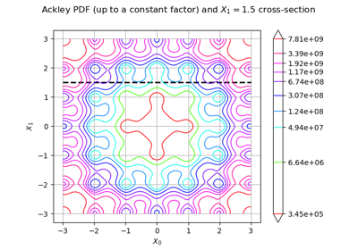
The Ackley test case is a real function defined in dimension where
is an integer.
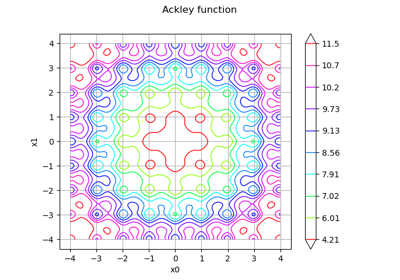
The Ackley function is defined by the equation:
for any . However, we consider the smaller interval
in this example, for visual purposes.
We use the dimension with the parameters
,
,
.
The solution is
where
References
Adorio, E. P., & Diliman, U. P. MVF - Multivariate Test Functions Library in C for Unconstrained Global Optimization (2005). Retrieved June 2013, from http://www.geocities.ws/eadorio/mvf.pdf.
Molga, M., & Smutnicki, C. Test functions for optimization needs (2005). Retrieved June 2013, from http://www.zsd.ict.pwr.wroc.pl/files/docs/functions.pdf.
Back, T. (1996). Evolutionary algorithms in theory and practice: evolution strategies, evolutionary programming, genetic algorithms. Oxford University Press on Demand.
API documentation
- class AckleyModel
Data class for the Ackley test function.
Examples
>>> from openturns.usecases import ackley_function
>>> # Load the Ackley model
>>> am = ackley_function.AckleyModel()
- Attributes:
- dimThe dimension of the problem
dim=2.
- aConstant
.
- bConstant
.
- cConstant
.
- modelPythonFunction, the Ackley function.
- lowerboundPoint in dimension dim.
Default is -15.0 for each dimension.
- upperboundPoint in dimension dim.
Default is +15.0 for each dimension.
- x0Point
The global minimum
.
 OpenTURNS

