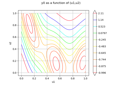
The Branin test case
Introduction
The Branin function is defined in 2 dimensions based on the functions :
and :
Finally, the Branin function is the composition of the two previous functions:
for any .
There are three global minimas:
and :
where the function value is:
We assume that the output of the Branin function is noisy, with a gaussian noise. In other words, the objective function is:
where is a Gaussian random variable with null mean and standard deviation
.
References
Dixon, L. C. W., & Szego, G. P. (1978). The global optimization problem: an introduction. Towards global optimization, 2, 1-15.
Forrester, A., Sobester, A., & Keane, A. (2008). Engineering design via surrogate modelling: a practical guide. Wiley.
Global Optimization Test Problems. Retrieved June 2013, from http://www-optima.amp.i.kyoto-u.ac.jp/member/student/hedar/Hedar_files/TestGO.htm.
Molga, M., & Smutnicki, C. Test functions for optimization needs (2005), from https://robertmarks.org/Classes/ENGR5358/Papers/functions.pdf.
Picheny, V., Wagner, T., & Ginsbourger, D. (2012). A benchmark of kriging-based infill criteria for noisy optimization.
API documentation
- class BraninModel
Data class for the Branin test function.
Examples
>>> from openturns.usecases import branin_function
>>> # Load the Branin model
>>> bm = branin_function.BraninModel()
- Attributes:
- dimThe dimension of the problem
dim=2.
- modelthe Branin function
- trueNoiseFunctionConstant, small noise
.
- noiseModelThe noise function
- lowerboundPoint in dimension dim.
Default is 0.0 for each dimension.
- upperboundPoint in dimension dim.
Default is 1.0 for each dimension.
- xexact1Point
First minima location
.
- xexact2Point
Second minima location
.
- xexact3Point
Third minima location
.
- xexactSample
All global minimas location gathered.
 OpenTURNS

