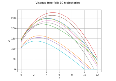
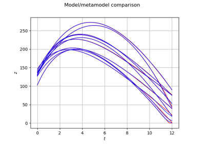
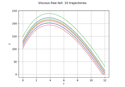
A viscous free fall example¶

Introduction¶

We consider an object inside a vertical cylinder which contains a viscous fluid. The fluid generates a drag force which limits the speed of the solid and we assume that the force depends linearily on the object speed:

$m \frac{dv}{dt} = - m g - c v$

for any $t \in [0, t_{max}]$ where:

$v$ is the speed $[m/s]$ ,
$t$ is the time $[s]$ ,
$t_{max}$ is the maximum time $[s]$ ,
$g = 9.81$ is the gravitational acceleration $[m.s^{-2}]$ ,
$m$ is the mass $[kg]$ ,
$c$ is the linear drag coefficient $[kg.s^{-1}]$ .

The exact solution of the previous differential equation is:

$z(t) = z_0 + v_{inf} t + \tau (v_0 - v_{inf})\left(1 - e^{-\frac{t}{\tau}}\right)$

for any $t \in [0, t_{max}]$

where:

$z$ is the altitude above the surface $[m]$ ,
$z_0$ is the initial altitude $[m]$ ,
$v_0$ is the initial speed (upward) $[m.s^{-1}]$ ,
$v_{inf}$ is the limit speed $[m.s^{-1}]$ :

$v_{inf}=-\frac{m g}{c}$

$\tau$ is time caracteristic $[s]$ :

$\tau=\frac{m}{c}.$

The stationnary speed limit at infinite time is equal to $v_{inf}$ :

$\lim_{t\rightarrow+\infty} v(t)= v_{inf}.$

When there is no drag, i.e. when $c=0$ , the trajectory depends quadratically on $t$ :

z(t) = z_0 + v_0 t -g t^2

for any $t \in [0, t_{max}]$ .

Furthermore when the solid touches the ground, we ensure that the altitude remains nonnegative i.e. the final altitude is:

$y(t) = \max(z(t),0)$

for any $t \in [0, t_{max}]$ .

Probabilistic model¶

The parameters $z_0$ , $v_0$ , $m$ and $c$ are probabilistic:

$z_0 \sim \mathcal{U}(100, 150)$ ,
$v_0 \sim \mathcal{N}(55, 10)$ ,
$m \sim \mathcal{N}(80, 8)$ ,
$c \sim \mathcal{U}(0, 30)$ .

References¶

Steven C. Chapra. Applied numerical methods with Matlab for engineers and scientists, Third edition. 2012. Chapter 7, “Optimization”, p.182.

API documentation¶

class ViscousFreeFall

Data class for the viscous free fall.

Examples

>>> from openturns.usecases import viscous_free_fall
>>> # Load the viscous free fall example
>>> vff = viscous_free_fall.ViscousFreeFall()

Attributes:

dimThe dimension of the problem: dim=4.
outputDimensionThe output dimension of the problem: outputDimension=1.
tminConstant: Minimum time, tmin = 0.0
tmaxConstant: Maximum time, tmax = 12.0
gridsizeConstant: Number of time steps, gridsize = 100.
meshIntervalMesher
verticesVertices of the mesh
distZ0Uniform distribution of the initial altitude: ot.Uniform(100.0, 150.0)
distV0Normal distribution of the initial speed: ot.Normal(55.0, 10.0)
distMNormal distribution of the mass: ot.Normal(80.0, 8.0)
distCUniform distribution of the drag: ot.Uniform(0.0, 30.0)
distributionJointDistribution: The joint distribution of the input parameters.
modelPythonPointToFieldFunction, the exact solution of the fall: ot.PythonPointToFieldFunction(dim, mesh, outputDimension, AltiFunc)