FAST
- class FAST(*args)
Fourier Amplitude Sensitivity Testing (FAST).
Refer to Sensitivity analysis by Fourier decomposition.
- Parameters:
- model
Function Definition of the model to analyse.
- distribution
Distribution Contains the distributions of each model’s input. Its dimension must be equal to the number of inputs.
- Nint,
Size of the sample from which the Fourier series are calculated. It represents the length of the discretization of the s-space.
- Nrint,
, optional
Number of resamplings. The extended FAST method involves a part of randomness in the computation of the indices. So it can be asked to realize the procedure Nr times and then to calculate the arithmetic means of the results over the Nr estimates.
- Mint,
, optional
Interference factor usually equal to 4 or higher. It corresponds to the truncation level of the Fourier series, i.e. the number of harmonics that are retained in the decomposition.
- model
Notes
FAST is a sensitivity analysis method which is based upon the ANOVA decomposition of the variance of the model response
, the latter being represented by its Fourier expansion.
is an input random vector of
independent components.
OpenTURNS implements the extended FAST method consisting in computing alternately the first order and the total-effect indices of each input. This approach, widely described in the paper by [saltelli1999], relies upon a Fourier decomposition of the model response. Its key idea is to recast this representation as a function of a scalar parameter
, by defining parametric curves
exploring the support of the input random vector
.
Then the Fourier expansion of the model response is:
where
and
are Fourier coefficients whose estimates are:
The first order indices are estimated by:
and the total order indices by:
where
is the total variance,
the portion of
arising from the uncertainty of the
input and
is the part of the variance due to all the inputs except the
input.
is the size of the sample using to compute the Fourier series and
is the interference factor. Saltelli et al. (1999) recommended to set
to a value in the range
.
is a set of integer frequencies assigned to each input
. The frequency associated with the input for which the sensitivity indices are computed, is set to the maximum admissible frequency satisfying the Nyquist criterion (which ensures to avoid aliasing effects):
In the paper by Saltelli et al. (1999), for high sample size, it is suggested that
.
Examples
>>> import openturns as ot
>>> ot.RandomGenerator.SetSeed(0)
>>> formula = ['sin(pi_*X1)+7*sin(pi_*X2)^2+0.1*(pi_*X3)^4*sin(pi_*X1)']
>>> model = ot.SymbolicFunction(['X1', 'X2', 'X3'], formula)
>>> distribution = ot.JointDistribution([ot.Uniform(-1.0, 1.0)] * 3)
>>> sensitivityAnalysis = ot.FAST(model, distribution, 101)
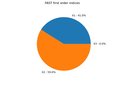
>>> print(sensitivityAnalysis.getFirstOrderIndices())
[0.311097,0.441786,0.000396837]
Methods
Get the block size.
Accessor to the FFT algorithm implementation.
getFirstOrderIndices([marginalIndex])Accessor to the first order indices.
getTotalOrderIndices([marginalIndex])Accessor to the total order indices.
setBlockSize(blockSize)Set the block size.
setFFTAlgorithm(fft)Accessor to the FFT algorithm implementation.
- __init__(*args)
- getBlockSize()
Get the block size.
- Returns:
- kpositive int
Size of each block the sample is split into, this allows one to save space while allowing multithreading, when available we recommend to use the number of available CPUs, set by default to 1.
- getFirstOrderIndices(marginalIndex=0)
Accessor to the first order indices.
- Parameters:
- marginalIndexint,
, optional
Index of the model’s marginal used to estimate the indices. By default, marginalIndex is equal to 0.
- marginalIndexint,
- Returns:
- indices
Point List of the first order indices of all the inputs.
- indices
- getTotalOrderIndices(marginalIndex=0)
Accessor to the total order indices.
- Parameters:
- marginalIndexint,
, optional
Index of the model’s marginal used to estimate the indices. By default, marginalIndex is equal to 0.
- marginalIndexint,
- Returns:
- indices
Point List of the total-effect order indices of all the inputs.
- indices
- setBlockSize(blockSize)
Set the block size.
- Parameters:
- kpositive int
Size of each block the sample is split into, this allows one to save space while allowing multithreading, when available we recommend to use the number of available CPUs, set by default to
.
 OpenTURNS
