IteratedQuadrature
(Source code, png)

- class IteratedQuadrature(*args)
Multivariate integration algorithm.
- Parameters:
- univariateQuadrature
IntegrationAlgorithm By default, the integration algorithm is the Gauss-Kronrod algorithm (
GaussKronrod) with the parameters IteratedQuadrature-MaximumSubIntervals, IteratedQuadrature-MaximumError, IteratedQuadrature-Rule inResourceMap. Note that the default parametrisation of theGaussKronrodclass leads to a more precise evaluation of the integral but the cost is greater. It is recommended to increase the order of the quadratic rule and the number of sub intervals if the integrand or one of the bound functions is smooth but with many oscillations.
- univariateQuadrature
Notes
This class enables to approximate the following integral:
with
,
and
. For
, there is no bound functions
and
.
Examples
Create an iterated quadrature algorithm:
>>> import openturns as ot
>>> import math as m
>>> a = -m.pi
>>> b = m.pi
>>> f = ot.SymbolicFunction(['x', 'y'], ['1+cos(x)*sin(y)'])
>>> l = [ot.SymbolicFunction(['x'], [' 2+cos(x)'])]
>>> u = [ot.SymbolicFunction(['x'], ['-2-cos(x)'])]
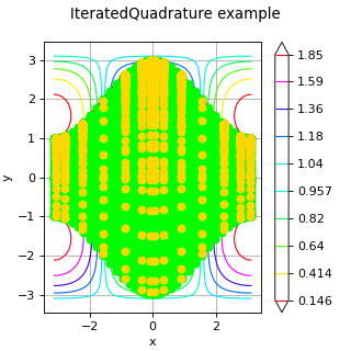
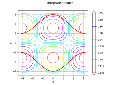
Draw the graph of the integrand and the bounds:
>>> g = ot.Graph('Integration nodes', 'x', 'y', True, 'upper right')
>>> g.add(f.draw([a,a],[b,b]))
>>> curve = l[0].draw(a, b).getDrawable(0)
>>> curve.setLineWidth(2)
>>> curve.setColor('red')
>>> g.add(curve)
>>> curve = u[0].draw(a, b).getDrawable(0)
>>> curve.setLineWidth(2)
>>> curve.setColor('red')
>>> g.add(curve)
Evaluate the integral with high precision:
>>> Iref = ot.IteratedQuadrature(ot.GaussKronrod(100000, 1e-13, ot.GaussKronrodRule(ot.GaussKronrodRule.G11K23))).integrate(f, a, b, l, u)
Evaluate the integral with the default GaussKronrod algorithm, and get evaluation points:
>>> f = ot.MemoizeFunction(f)
>>> I1 = ot.IteratedQuadrature(ot.GaussKronrod()).integrate(f, a, b, l, u)
>>> sample1 = f.getInputHistory()
>>> print(I1)
[-25.132...]
>>> n_evals = sample1.getSize()
>>> print(n_evals)
2116
>>> err = abs(100.0*(1.0-I1[0]/Iref[0]))
>>> print(err)
2.2...e-14
>>> cloud = ot.Cloud(sample1)
>>> cloud.setPointStyle('fcircle')
>>> cloud.setColor('green')
>>> g.add(cloud)
>>> f.clearHistory()
Evaluate the integral with the default IteratedQuadrature algorithm:
>>> I2 = ot.IteratedQuadrature().integrate(f, a, b, l, u)
>>> sample2 = f.getInputHistory()
>>> print(I2)
[-25.132...]
>>> n_evals = sample2.getSize()
>>> print(n_evals)
5236
>>> err = abs(100.0*(1.0-I2[0]/Iref[0]))
>>> print(err)
4.6...e-10
>>> cloud = ot.Cloud(sample2)
>>> cloud.setPointStyle('fcircle')
>>> cloud.setColor('gold')
>>> g.add(cloud)
Methods
Accessor to the underlying 1D integration algorithm.
Accessor to the object's name.
getName()Accessor to the object's name.
hasName()Test if the object is named.
integrate(*args)Evaluation of the integral of
on a domain.
setAlgorithm(algorithm)Set the underlying 1D integration algorithm.
setName(name)Accessor to the object's name.
- __init__(*args)
- getAlgorithm()
Accessor to the underlying 1D integration algorithm.
- Returns:
- algo
IntegrationAlgorithm The 1D integration algorithm used recursively over the dimensions of the integration domain.
- algo
- getClassName()
Accessor to the object’s name.
- Returns:
- class_namestr
The object class name (object.__class__.__name__).
- getName()
Accessor to the object’s name.
- Returns:
- namestr
The name of the object.
- hasName()
Test if the object is named.
- Returns:
- hasNamebool
True if the name is not empty.
- integrate(*args)
Evaluation of the integral of
on a domain.
- Available usages:
integrate(f, interval)
integrate(f, a, b, lowerBoundFunctions, upperBoundFunctions)
- Parameters:
- f
Function, The integrand function.
- interval
Interval, The integration domain.
- a,bfloat
Bounds of the integration interval of the first scalar input
- lowerBoundFunctions, upperBoundFunctionslist of
Function List of
functions
and
where
defining the integration domain as defined above. The bound functions can cross each other.
- f
- Returns:
- value
Point Approximation of the integral.
- value
- setAlgorithm(algorithm)
Set the underlying 1D integration algorithm.
- Parameters:
- algo
IntegrationAlgorithm The 1D integration algorithm used recursively over the dimensions of the integration domain.
- algo
- setName(name)
Accessor to the object’s name.
- Parameters:
- namestr
The name of the object.
 OpenTURNS
