Note

Go to the end to download the full example code.

Estimate a GEV on the Fremantle sea-levels data¶

In this example, we illustrate various techniques of extreme value modeling applied to the annual maximum sea-levels recorded at Fremantle, near Perth, western Australia, over the period 1897-1989. Readers should refer to [coles2001] to get more details.

We illustrate techniques to:

estimate a stationary and a non stationary GEV depending on time or on the covariates (time, SOI),
estimate a return level,

using:

the log-likelihood function,
the profile log-likelihood function.

We also illustrate the modelling with covariates.

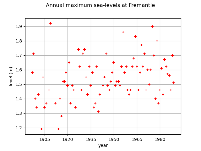
First, we load the Fremantle dataset of the annual maximum sea-levels. We start by looking at them through time. The data also contain the annual mean value of the Southern Oscillation Index (SOI), which is a proxy for meteorological volatility due to effects such as El Nino.

import openturns as ot
import openturns.viewer as otv
from openturns.usecases import coles

data = coles.Coles().fremantle
print(data[:5])
graph = ot.Graph(
    "Annual maximum sea-levels at Fremantle", "year", "level (m)", True, ""
)
cloud = ot.Cloud(data[:, :2])
cloud.setColor("red")
graph.add(cloud)
graph.setIntegerXTick(True)
view = otv.View(graph)

    [ Year     SeaLevel SOI      ]
: [ 1897        1.58    -0.67  ]
: [ 1898        1.71     0.57  ]
: [ 1899        1.4      0.16  ]
: [ 1900        1.34    -0.65  ]
: [ 1901        1.43     0.06  ]

We select the sea-levels column.

sample = data[:, 1]

Stationary GEV modeling via the log-likelihood function

We first assume that the dependence through time is negligible, so we first model the data as independent observations over the observation period. We estimate the parameters of the GEV distribution by maximizing the log-likelihood of the data.

factory = ot.GeneralizedExtremeValueFactory()
result_LL = factory.buildMethodOfLikelihoodMaximizationEstimator(sample)

We get the fitted GEV and its parameters $(\hat{\mu}, \hat{\sigma}, \hat{\xi})$ .

fitted_GEV = result_LL.getDistribution()
desc = fitted_GEV.getParameterDescription()
param = fitted_GEV.getParameter()
print(", ".join([f"{p}: {value:.3f}" for p, value in zip(desc, param)]))

mu: 1.482, sigma: 0.141, xi: -0.217

We get the asymptotic distribution of the estimator $(\hat{\mu}, \hat{\sigma}, \hat{\xi})$ . In that case, the asymptotic distribution is normal.

parameterEstimate = result_LL.getParameterDistribution()
print("Asymptotic distribution of the estimator : ")
print(parameterEstimate)

Asymptotic distribution of the estimator :
Normal(mu = [1.48231,0.141241,-0.217052], sigma = [0.0176728,0.0105976,0.0776361], R = [[  1         0.15748  -0.482101 ]
 [  0.15748   1        -0.411378 ]
 [ -0.482101 -0.411378  1        ]])

We get the covariance matrix and the standard deviation of $(\hat{\mu}, \hat{\sigma}, \hat{\xi})$ .

print("Cov matrix = \n", parameterEstimate.getCovariance())
print("Standard dev = ", parameterEstimate.getStandardDeviation())

Cov matrix =
 [[  0.000312329  2.94943e-05 -0.000661467 ]
 [  2.94943e-05  0.000112309 -0.000338463 ]
 [ -0.000661467 -0.000338463  0.00602736  ]]
Standard dev =  [0.0176728,0.0105976,0.0776361]

We get the marginal confidence intervals of order 0.95.

order = 0.95
for i in range(3):
    ci = parameterEstimate.getMarginal(i).computeBilateralConfidenceInterval(order)
    print(desc[i] + ":", ci)

mu: [1.44767, 1.51694]
sigma: [0.12047, 0.162012]
xi: [-0.369216, -0.0648881]

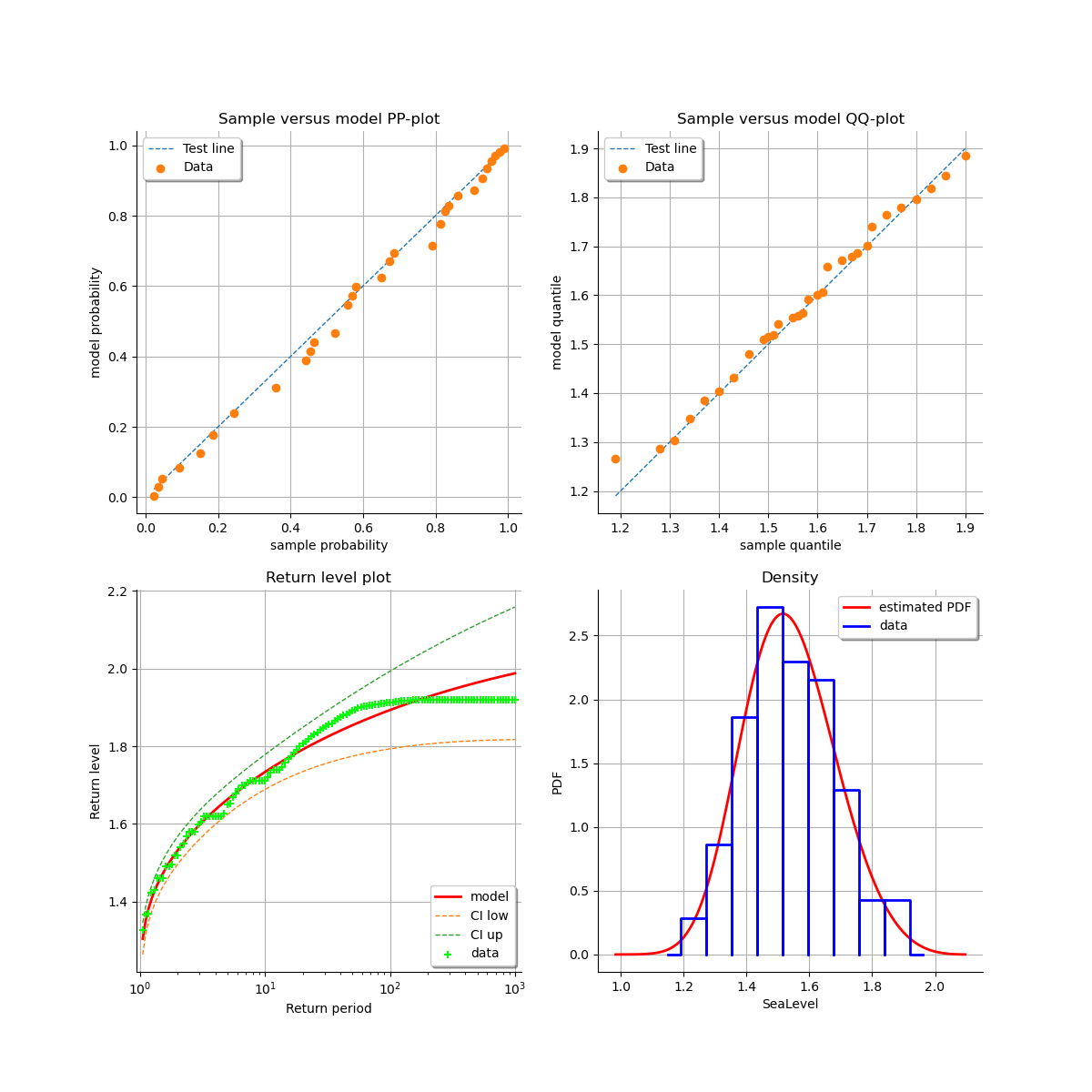
At last, we can validate the inference result thanks the 4 usual diagnostic plots:

the probability-probability pot,
the quantile-quantile pot,
the return level plot,
the empirical distribution function.

validation = ot.GeneralizedExtremeValueValidation(result_LL, sample)
graph = validation.drawDiagnosticPlot()
view = otv.View(graph)

, Sample versus model PP-plot, Sample versus model QQ-plot, Return level plot, Density

Stationary GEV modeling via the profile log-likelihood function

Now, we use the profile log-likehood function rather than log-likehood function to estimate the parameters of the GEV.

result_PLL = factory.buildMethodOfXiProfileLikelihoodEstimator(sample)

The following graph allows one to get the profile log-likelihood plot. It also indicates the optimal value of $\xi$ , the maximum profile log-likelihood and the confidence interval for $\xi$ of order 0.95 (which is the default value).

order = 0.95
result_PLL.setConfidenceLevel(order)
view = otv.View(result_PLL.drawProfileLikelihoodFunction())

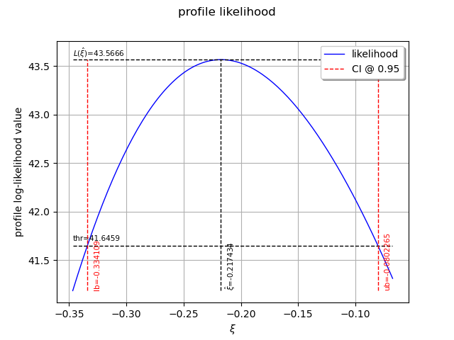
We can get the numerical values of the confidence interval: it appears to be a bit smaller than the interval obtained with the log-likelihood function. Note that if the order requested is too high, the confidence interval might not be calculated because one of its bound is out of the definition domain of the log-likelihood function.

try:
    print("Confidence interval for xi = ", result_PLL.getParameterConfidenceInterval())
except Exception as ex:
    print(type(ex))
    pass

Confidence interval for xi =  [-0.334109, -0.0802265]

Return level estimate from the estimated stationary GEV

We estimate the $m$ -block return level $z_m$ : it is computed as a particular quantile of the GEV model estimated using the log-likelihood function. We just have to use the maximum log-likelihood estimator built in the previous section.

As the data are annual sea-levels, each block corresponds to one year: the 10-year return level corresponds to $m=10$ and the 100-year return level corresponds to $m=100$ .

The method provides the asymptotic distribution of the estimator $\hat{z}_m$ which mean is the return-level estimate.

zm_10 = factory.buildReturnLevelEstimator(result_LL, 10.0)
return_level_10 = zm_10.getMean()
print("Maximum log-likelihood function : ")
print(f"10-year return level = {return_level_10}")
return_level_ci10 = zm_10.computeBilateralConfidenceInterval(0.95)
print(f"CI = {return_level_ci10}")

Maximum log-likelihood function :
10-year return level = [1.73376]
CI = [1.68892, 1.7786]

zm_100 = factory.buildReturnLevelEstimator(result_LL, 100.0)
return_level_100 = zm_100.getMean()
print(f"100-year return level = {return_level_100}")
return_level_ci100 = zm_100.computeBilateralConfidenceInterval(0.95)
print(f"CI = {return_level_ci100}")

100-year return level = [1.89328]
CI = [1.79336, 1.99319]

Return level estimate via the profile log-likelihood function of a stationary GEV

We can estimate the $m$ -block return level $z_m$ directly from the data using the profile likelihood with respect to $z_m$ .

result_zm_10_PLL = factory.buildReturnLevelProfileLikelihoodEstimator(sample, 10.0)
zm_10_PLL = result_zm_10_PLL.getParameter()
print(f"10-year return level (profile) = {zm_10_PLL}")

10-year return level (profile) = 1.7337304564424916

We can get the confidence interval of $z_m$ : once more, it appears to be a bit smaller than the interval obtained from the log-likelihood function. As for the confidence interval of $\xi$ , depending on the order requested, the interval might not be calculated.

result_zm_10_PLL.setConfidenceLevel(0.95)
try:
    return_level_ci10 = result_zm_10_PLL.getParameterConfidenceInterval()
except Exception as ex:
    print(type(ex))
    pass
print("Maximum profile log-likelihood function : ")
print(f"CI={return_level_ci10}")

Maximum profile log-likelihood function :
CI=[1.69343, 1.78619]

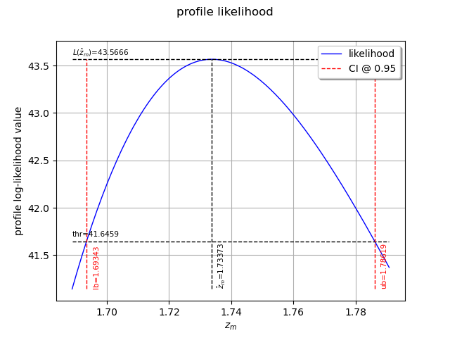
We can also plot the profile log-likelihood function and get the confidence interval, the optimal value of $z_m$ and its confidence interval.

view = otv.View(result_zm_10_PLL.drawProfileLikelihoodFunction())

Non stationary GEV modeling via the log-likelihood function

If we look at the data carefully, we see that the pattern of variation has not remained constant over the observation period. There is an increase in the data through time. We want to model this dependence because a slight increase in extreme sea-levels might have a significant impact on the safety of coastal flood defenses.

We have define the functional basis for each parameter of the GEV model. Even if we have the possibility to affect a time-varying model to each of the 3 parameters $(\mu, \sigma, \xi)$ , it is strongly recommended not to vary the parameter $\xi$ and to let it constant.

For numerical reasons, it is strongly recommended to normalize all the data as follows:

$\tau(t) = \dfrac{t-c}{d}$

where:

the CenterReduce method where $c = \dfrac{1}{n} \sum_{i=1}^n t_i$ is the mean time stamps and $d = \sqrt{\dfrac{1}{n} \sum_{i=1}^n (t_i-c)^2}$ is the standard deviation of the time stamps;
the MinMax method where $c = t_1$ is the initial time and $d = t_n-t_1$ the final time;
the None method where $c = 0$ and $d = 1$ : in that case, data are not normalized.

We suppose that $\mu$ is linear in time, and that the other parameters remain constant:

$\begin{align*} \mu(t) & = \beta_1 + \beta_2\tau(t) \\ \sigma(t) & = \beta_3 \\ \xi(t) & = \beta_4 \end{align*}$

constant = ot.SymbolicFunction(["t"], ["1.0"])
basis = ot.Basis([constant, ot.SymbolicFunction(["t"], ["t"])])
# basis for mu, sigma, xi
muIndices = [0, 1]  # linear
sigmaIndices = [0]  # stationary
xiIndices = [0]  # stationary

timeStamps = data[:, 0]

We can now estimate the list of coefficients $\vect{\beta} = (\beta_1, \beta_2, \beta_3, \beta_4)$ using the log-likelihood of the data.

We test the 3 normalizing methods and both initial points in order to evaluate their impact on the results. We can see that:

both normalization methods lead to the same result for $\beta_1$ , $\beta_3$ and $\beta_4$ (note that $\beta_2$ depends on the normalization function),
both initial points lead to the same result when the data have been normalized,
it is very important to normalize all the data: if not, the result strongly depends on the initial point and it differs from the result obtained with normalized data. The results are not optimal in that case since the associated log-likelihood are much smaller than those obtained with normalized data.

print("Linear mu(t) model:")
for normMeth in ["MinMax", "CenterReduce", "None"]:
    for initPoint in ["Gumbel", "Static"]:
        print(f"normMeth = {normMeth}, initPoint = {initPoint}")
        # The ot.Function() is the identity function.
        result = factory.buildTimeVarying(
            sample,
            timeStamps,
            basis,
            muIndices,
            sigmaIndices,
            xiIndices,
            ot.Function(),
            ot.Function(),
            ot.Function(),
            initPoint,
            normMeth,
        )
        beta = result.getOptimalParameter()
        print(f"beta = {beta}")
        print(f"Max log-likelihood = {result.getLogLikelihood()}")

Linear mu(t) model:
normMeth = MinMax, initPoint = Gumbel
beta = [1.3821,0.187126,0.124302,-0.124882]
Max log-likelihood = 49.912792759600805
normMeth = MinMax, initPoint = Static
beta = [1.38227,0.186899,0.124343,-0.125475]
Max log-likelihood = 49.91281020707175
normMeth = CenterReduce, initPoint = Gumbel
beta = [1.48016,0.0541552,0.124306,-0.124888]
Max log-likelihood = 49.91279529325528
normMeth = CenterReduce, initPoint = Static
beta = [1.48022,0.0541103,0.124358,-0.125708]
Max log-likelihood = 49.912796771958874
normMeth = None, initPoint = Gumbel
beta = [1.47155,1.67803e-05,0.211226,0.0876902]
Max log-likelihood = 26.490076768443522
normMeth = None, initPoint = Static
beta = [1.4823,1.34614e-09,0.141241,-0.217051]
Max log-likelihood = 43.566619143025775

According to the previous results, we choose the MinMax normalization method and the Gumbel initial point. This initial point is cheaper than the Static one as it requires no optimization computation.

result_NonStatLL = factory.buildTimeVarying(
    sample,
    timeStamps,
    basis,
    muIndices,
    sigmaIndices,
    xiIndices,
    ot.Function(),
    ot.Function(),
    ot.Function(),
    "Gumbel",
    "MinMax",
)
beta = result_NonStatLL.getOptimalParameter()
print(f"beta = {beta}")
print(f"mu(t) = {beta[0]:.4f} + {beta[1]:.4f} * tau(t)")
print(f"sigma = {beta[2]:.4f}")
print(f"xi = {beta[3]:.4f}")

beta = [1.3821,0.187126,0.124302,-0.124882]
mu(t) = 1.3821 + 0.1871 * tau(t)
sigma = 0.1243
xi = -0.1249

You can get the expression of the normalizing function $t \mapsto \tau(t)$ :

normFunc = result_NonStatLL.getNormalizationFunction()
print("Function tau(t): ", normFunc)
print("c = ", normFunc.getEvaluation().getImplementation().getCenter()[0])
print("1/d = ", normFunc.getEvaluation().getImplementation().getLinear()[0, 0])

Function tau(t):  class=LinearFunction name=Unnamed implementation=class=LinearEvaluation name=Unnamed center=[1897] constant=[0] linear=[[ 0.0108696 ]]
c =  1897.0
1/d =  0.010869565217391304

You can get the function $t \mapsto \vect{\theta}(t)$ where $\vect{\theta}(t) = (\mu(t), \sigma(t), \xi(t))$ .

functionTheta = result_NonStatLL.getParameterFunction()

We get the asymptotic distribution of $\vect{\beta}$ to compute some confidence intervals of the estimates, for example of order $p = 0.95$ .

dist_beta = result_NonStatLL.getParameterDistribution()
confidence_level = 0.95
for i in range(beta.getSize()):
    lower_bound = dist_beta.getMarginal(i).computeQuantile((1 - confidence_level) / 2)[
        0
    ]
    upper_bound = dist_beta.getMarginal(i).computeQuantile((1 + confidence_level) / 2)[
        0
    ]
    print(
        "Conf interval for beta_"
        + str(i + 1)
        + " = ["
        + str(lower_bound)
        + "; "
        + str(upper_bound)
        + "]"
    )

Conf interval for beta_1 = [1.3760619004522263; 1.3881370574735519]
Conf interval for beta_2 = [0.17703896126886012; 0.19721356765581052]
Conf interval for beta_3 = [0.12188407872826672; 0.1267190556645434]
Conf interval for beta_4 = [-0.142994007106013; -0.10677058768572634]

In order to compare different modelings, we get the optimal log-likelihood of the data for both stationary and non stationary models. The difference is significant enough to be in favor of the non stationary model.

print("Max log-likelihood: ")
print("Stationary model =  ", result_LL.getLogLikelihood())
print("Non stationary linear mu(t) model =  ", result_NonStatLL.getLogLikelihood())

Max log-likelihood:
Stationary model =   43.566611777651026
Non stationary linear mu(t) model =   49.912792759600805

In order to draw some diagnostic plots similar to those drawn in the stationary case, we refer to the following result: if $Z_t$ is a non stationary GEV model parametrized by $(\mu(t), \sigma(t), \xi(t))$ , then the standardized variables $\hat{Z}_t$ defined by:

$\hat{Z}_t = \dfrac{1}{\xi(t)} \log \left[1+ \xi(t)\left( \dfrac{Z_t-\mu(t)}{\sigma(t)} \right)\right]$

have the standard Gumbel distribution which is the GEV model with $(\mu, \sigma, \xi) = (0, 1, 0)$ .

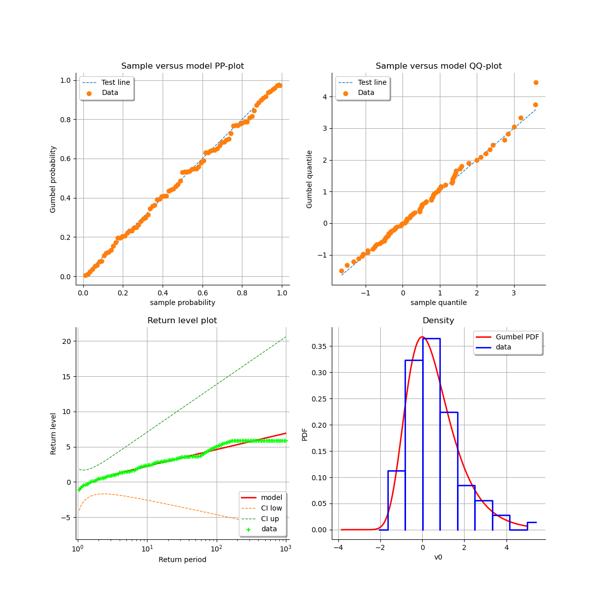
As a result, we can validate the inference result thanks the 4 usual diagnostic plots:

the probability-probability pot,
the quantile-quantile pot,
the return level plot,
the data histogram and the density of the fitted model.

using the transformed data compared to the Gumbel model. We can see that the adequation is better than with the stationary model.

graph = result_NonStatLL.drawDiagnosticPlot()
view = otv.View(graph)

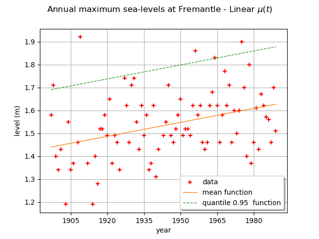
We can draw the mean function $t \mapsto \Expect{\mbox{GEV}(t)}$ . Be careful, it is not the function $t \mapsto \mu(t)$ . As a matter of fact, the mean is defined for $\xi <1$ only and in that case, for $\xi \neq 0$ , we have:

$\Expect{\mbox{GEV}(t)} = \mu(t) + \dfrac{\sigma(t)}{\xi(t)} (\Gamma(1-\xi(t))-1)$

and for $\xi = 0$ , we have:

$\Expect{\mbox{GEV}(t)} = \mu(t) + \sigma(t)\gamma$

where $\gamma$ is the Euler constant.

We can also draw the function $t \mapsto q_p(t)$ where $q_p(t)$ is the quantile of order $p$ of the GEV distribution at time $t$ . Here, $\mu(t)$ is a linear function and the other parameters are constant, so the mean and the quantile functions are also linear functions.

graph = ot.Graph(
    r"Annual maximum sea-levels at Fremantle - Linear $\mu(t)$",
    "year",
    "level (m)",
    True,
    "",
)
graph.setIntegerXTick(True)
# data
cloud = ot.Cloud(data[:, :2])
cloud.setColor("red")
graph.add(cloud)
# mean function
meandata = [
    result_NonStatLL.getDistribution(t).getMean()[0] for t in data[:, 0].asPoint()
]
curve_meanPoints = ot.Curve(data[:, 0].asPoint(), meandata)
graph.add(curve_meanPoints)
# quantile function
graphQuantile = result_NonStatLL.drawQuantileFunction(0.95)
drawQuant = graphQuantile.getDrawable(0)
drawQuant = graphQuantile.getDrawable(0)
drawQuant.setLineStyle("dashed")
graph.add(drawQuant)
graph.setLegends(["data", "mean function", "quantile 0.95  function"])
graph.setLegendPosition("lower right")
view = otv.View(graph)

$Annual maximum sea-levels at Fremantle - Linear $\mu(t)$$

At last, we can test the validity of the stationary model $\mathcal{M}_0$ relative to the model with time varying parameters $\mathcal{M}_1$ . The model $\mathcal{M}_0$ is parametrized by $(\beta_1, \beta_3, \beta_4)$ and the model $\mathcal{M}_1$ is parametrized by $(\beta_1, \beta_2, \beta_3, \beta_4)$ : so we have $\mathcal{M}_0 \subset \mathcal{M}_1$ .

We use the Likelihood Ratio test. The null hypothesis is the stationary model $\mathcal{M}_0$ . The Type I error $\alpha$ is taken equal to 0.05.

This test confirms that the dependence through time is not negligible: it means that the linear $\mu(t)$ component explains a large variation in the data.

llh_LL = result_LL.getLogLikelihood()
llh_NonStatLL = result_NonStatLL.getLogLikelihood()
modelM0_Nb_param = 3
modelM1_Nb_param = 4
resultLikRatioTest = ot.HypothesisTest.LikelihoodRatioTest(
    modelM0_Nb_param, llh_LL, modelM1_Nb_param, llh_NonStatLL, 0.05
)
accepted = resultLikRatioTest.getBinaryQualityMeasure()
print(
    f"Hypothesis H0 (stationary model) vs H1 (linear mu(t) model):  accepted ? = {accepted}"
)

Hypothesis H0 (stationary model) vs H1 (linear mu(t) model):  accepted ? = False

We detail the statistics of the Likelihood Ratio test: the deviance statistics $\mathcal{D}_p$ follows a $\chi^2_1$ distribution. The model $\mathcal{M}_0$ is rejected if the deviance statistics estimated on the data is greater than the threshold $c_{\alpha}$ or if the p-value is less than the Type I error $\alpha = 0.05$ .

print(f"Dp={resultLikRatioTest.getStatistic():.2f}")
print(f"alpha={resultLikRatioTest.getThreshold():.2f}")
print(f"p-value={resultLikRatioTest.getPValue():.2f}")

Dp=12.69
alpha=0.05
p-value=0.00

We can perform the same study with a quadratic model for $\mu(t)$ or a linear model for $\mu(t)$ and $\sigma(t)$ :

$\begin{align*} \mu(t) & = \beta_1 + \beta_2 \tau(t) + \beta_3\tau(t)^2 \\ \sigma(t) & = \beta_4 \\ \xi(t) & = \beta_5 \end{align*}$

or

$\begin{align*} \mu(t) & = \beta_1 + \beta_2 \tau(t) \\ \sigma(t) & = \beta_3 + \beta_4\tau(t)\\ \xi(t) & = \beta_5 \end{align*}$

For each model, we give the log-likelihood values and we test the validity of each model with respect to the non stationary model where $\mu(t)$ is linear. We notice that there is no evidence to adopt a quadratic model for $\mu(t)$ nor a linear model for $\mu(t)$ and $\sigma(t)$ : the optimal log-likelihood for each model is very near the likelihood we obtained with a linear model for $\mu(t)$ only. It means that these both models do not bring significant improvements with respect to model tested before.

basis = ot.Basis(
    [constant, ot.SymbolicFunction(["t"], ["t"]), ot.SymbolicFunction(["t"], ["t^2"])]
)
result_NonStatLL_2 = factory.buildTimeVarying(
    sample,
    timeStamps,
    basis,
    [0, 1, 2],
    [0],
    [0],
    ot.Function(),
    ot.Function(),
    ot.Function(),
    "Gumbel",
    "MinMax",
)
result_NonStatLL_3 = factory.buildTimeVarying(
    sample,
    timeStamps,
    basis,
    [0, 1],
    [0, 1],
    [0],
    ot.Function(),
    ot.Function(),
    ot.Function(),
    "Gumbel",
    "MinMax",
)
print("Max log-likelihood = ")
print("Non stationary quadratic mu(t) model = ", result_NonStatLL_2.getLogLikelihood())
print(
    "Non stationary linear mu(t) and sigma(t) model = ",
    result_NonStatLL_3.getLogLikelihood(),
)
llh_LL = result_LL.getLogLikelihood()
llh_NonStatLL_2 = result_NonStatLL_2.getLogLikelihood()
llh_NonStatLL_3 = result_NonStatLL_3.getLogLikelihood()
resultLikRatioTest_2 = ot.HypothesisTest.LikelihoodRatioTest(
    4, llh_NonStatLL, 5, llh_NonStatLL_2, 0.05
)
resultLikRatioTest_3 = ot.HypothesisTest.LikelihoodRatioTest(
    4, llh_NonStatLL, 5, llh_NonStatLL_3, 0.05
)
accepted_2 = resultLikRatioTest_2.getBinaryQualityMeasure()
accepted_3 = resultLikRatioTest_3.getBinaryQualityMeasure()
print(
    f"Hypothesis H0 (linear mu(t) model) vs H1 (quadratic mu(t) model):  accepted ? = {accepted_2}"
)
print(
    f"Hypothesis H0 (linear mu(t) model) vs H1 (linear mu(t) and sigma(t) model):  accepted ? = {accepted_3}"
)

Max log-likelihood =
Non stationary quadratic mu(t) model =  50.654392295132084
Non stationary linear mu(t) and sigma(t) model =  50.703072460849185
Hypothesis H0 (linear mu(t) model) vs H1 (quadratic mu(t) model):  accepted ? = True
Hypothesis H0 (linear mu(t) model) vs H1 (linear mu(t) and sigma(t) model):  accepted ? = True

Non stationary GEV modeling with the covariates Time and SOI

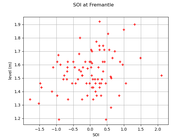
Extreme sea-levels can be unusually extreme during periods when the El Nino effect is active. Hence, we study a modeling that takes into account the dependence between the extreme sea-levels at Fremantle and the annual mean value of the Southern Oscillation Index (SOI) besides the temporal dependence. The following figure shows that the annual maximum sea-levels are generally greater when the value of SOI is high. It might be due to the time trend in the data for the sea-levels and the SOI (each one increases with time). But it can also be possible that the SOI explains some of the variation in annual maximum sea-levels after allowance for the time variation in the process.

graph = ot.Graph("SOI at Fremantle", "SOI", "level (m)", True, "")
cloud = ot.Cloud(data.getMarginal([2, 1]))
cloud.setColor("red")
graph.add(cloud)
view = otv.View(graph)

To consider this possibility, we study the model:

$\begin{align*} \mu(t) & = \beta_1 t + \beta_2 \mbox{SOI} + \beta_3 \\ \sigma(t) & = \beta_4 \\ \xi(t) & = \beta_5 \end{align*}$

We consider two covariates: the time and the SOI. We build the sample of the values of both covariates: $(t_i, \mbox{SOI}_i)_{1 \leq i \leq n}$ where $\mbox{SOI}_i = SOI(t_i)$ . The constant covariate is automatically added by the library if not specified in order to allow some of the GEV parameters to remain constant (ie independent of both covariates $(t, \mbox{SOI})$ ): this is the case for the $\sigma$ and $\xi$ parameters. This last constant covariate is associated to the third component of the covariates sample which now gathers the values $(t_i, \mbox{SOI}_i, 1)$ for $1 \leq i \leq n$ .

dataCovariates = data.getMarginal([0, 2])
print(dataCovariates[0:10])
result_Cov = factory.buildCovariates(sample, dataCovariates, [0, 1])

    [ Year    SOI     ]
: [ 1897      -0.67 ]
: [ 1898       0.57 ]
: [ 1899       0.16 ]
: [ 1900      -0.65 ]
: [ 1901       0.06 ]
: [ 1903       0.47 ]
: [ 1904       0.39 ]
: [ 1905      -1.78 ]
: [ 1906       0.2  ]
: [ 1908       0.28 ]

We check here that a third component has effectively been added to the covariates sample: see the added third column which is constant equal to 1.

print(result_Cov.getCovariates()[0:10])

    [ Year    SOI     v0      ]
: [ 1897      -0.67    1    ]
: [ 1898       0.57    1    ]
: [ 1899       0.16    1    ]
: [ 1900      -0.65    1    ]
: [ 1901       0.06    1    ]
: [ 1903       0.47    1    ]
: [ 1904       0.39    1    ]
: [ 1905      -1.78    1    ]
: [ 1906       0.2     1    ]
: [ 1908       0.28    1    ]

We get the optimal parameter $\vect{\beta}$ .

beta = result_Cov.getOptimalParameter()
print("beta = ", beta)

beta =  [0.00211399,0.0543691,-2.62594,0.12072,-0.149739]

We get here the function $(\vect{\beta}, t, \mbox{SOI}) \mapsto \vect{\theta} (\vect{\beta}, t, \mbox{SOI})$ where $\vect{\theta} = (\mu, \sigma, \xi)$ . We see that $\mu$ depends on the three covariates $(t, \mbox{SOI}, 1)$ and that $\sigma$ and $\xi$ depends only on the third one which is the constant one.

print(result_Cov.getParameterFunction())
print(f"beta = {beta}")
print(f"mu(t) = {beta[0]:.4f} *t + {beta[1]:.4f} * SOI(t) + {beta[2]:.4f}")
print(f"sigma = {beta[3]:.4f}")
print(f"xi = {beta[4]:.4f}")

ParametricEvaluation([muBeta0,muBeta1,muBeta2,sigmaBeta0,xiBeta0,y0,y1,y2]->[muBeta0 * y0 + muBeta1 * y1 + muBeta2 * y2,sigmaBeta0 * y2,xiBeta0 * y2], parameters positions=[0,1,2,3,4], parameters=[muBeta0 : 0.00211399, muBeta1 : 0.0543691, muBeta2 : -2.62594, sigmaBeta0 : 0.12072, xiBeta0 : -0.149739], input positions=[5,6,7])
beta = [0.00211399,0.0543691,-2.62594,0.12072,-0.149739]
mu(t) = 0.0021 *t + 0.0544 * SOI(t) + -2.6259
sigma = 0.1207
xi = -0.1497

We check here the normalizing function that has been used, which comes from the default method (the MinMax one).

print(result_Cov.getNormalizationFunction())

class=LinearFunction name=Unnamed implementation=class=LinearEvaluation name=Unnamed center=[1897,-1.78,0] constant=[0,0,0] linear=[[ 0.0108696 0         0         ]
 [ 0         0.25641   0         ]
 [ 0         0         1         ]]

We test this new model where $\mu(t,SOI)$ is modeled as a linear combination of the three covariates $(t, \mbox{SOI}, 1)$ against the model with the linear-trend only $\mu(t)$ . The maximized log-likelihood of this new model is 53.9, compared to 49.9 for the first model. Hence, the deviance statistics is equal to $D = 8.0$ , which is large when judged relative to a $\chi_1^2$ distribution. It provides evidence that the effect of SOI is influential on annual maximum sea-levels at Fremantle, even after the allowance for time-variation.

llh_cov = result_Cov.getLogLikelihood()
print("Max log-likelihood: ", llh_cov)
resultLikRatioTest_SOI = ot.HypothesisTest.LikelihoodRatioTest(
    4, llh_NonStatLL, 5, llh_cov, 0.05
)
print(f"Dp={resultLikRatioTest_SOI.getStatistic():.2f}")
accepted = resultLikRatioTest_SOI.getBinaryQualityMeasure()
print(
    f"Hypothesis H0 (linear-trend mu(t) model) vs H1 (linear-trend and SOI mu(t,SOI) model):  accepted ? = {accepted}"
)

Max log-likelihood:  53.89871913089317
Dp=7.97
Hypothesis H0 (linear-trend mu(t) model) vs H1 (linear-trend and SOI mu(t,SOI) model):  accepted ? = False

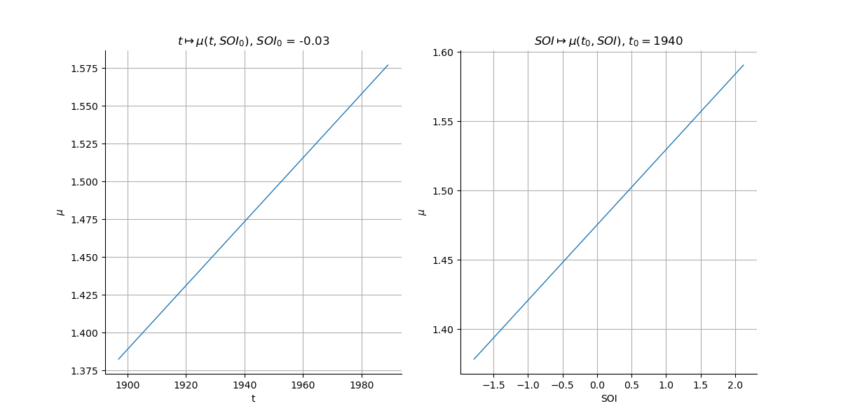
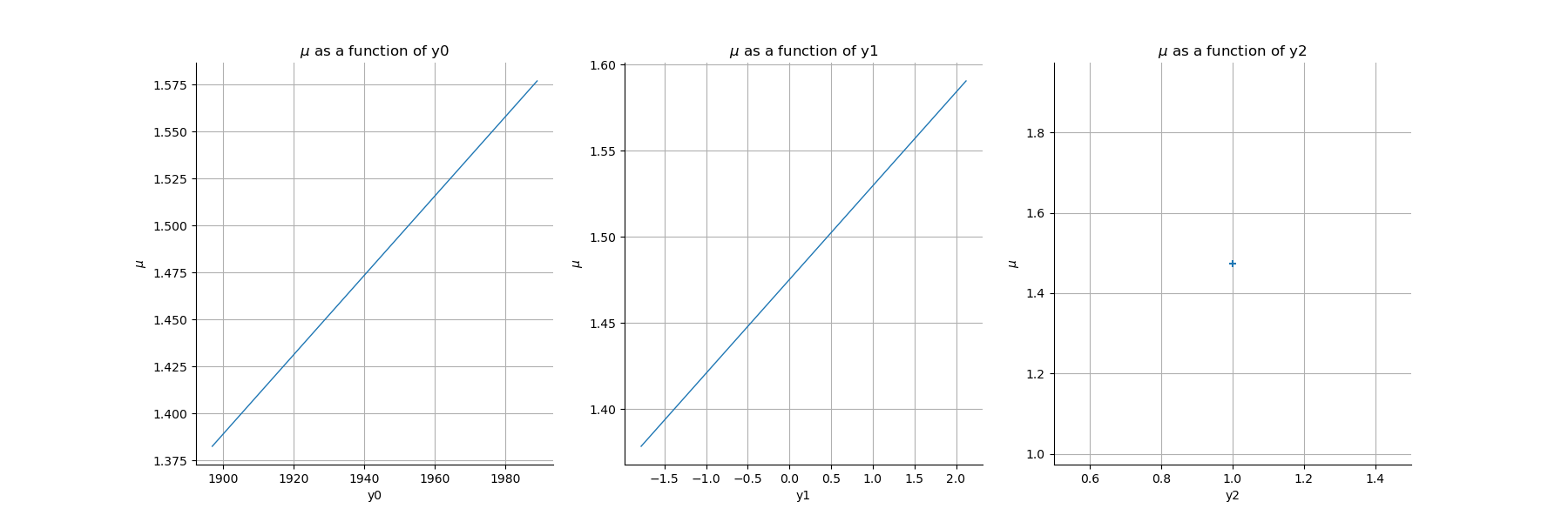
We plot here the graphs $t \mapsto \mu(t, \mbox{SOI}_0)$ where $\mbox{SOI}_0$ is a given value (the mean value of the sample if not specified), and $\mbox{SOI} \mapsto \mu(t_0, \mbox{SOI})$ where $t_0$ is a given time. Care: there are three covariates $(t, SOI, 1)$ for the reasons mentioned previously. Then the reference point must be of dimension 3.

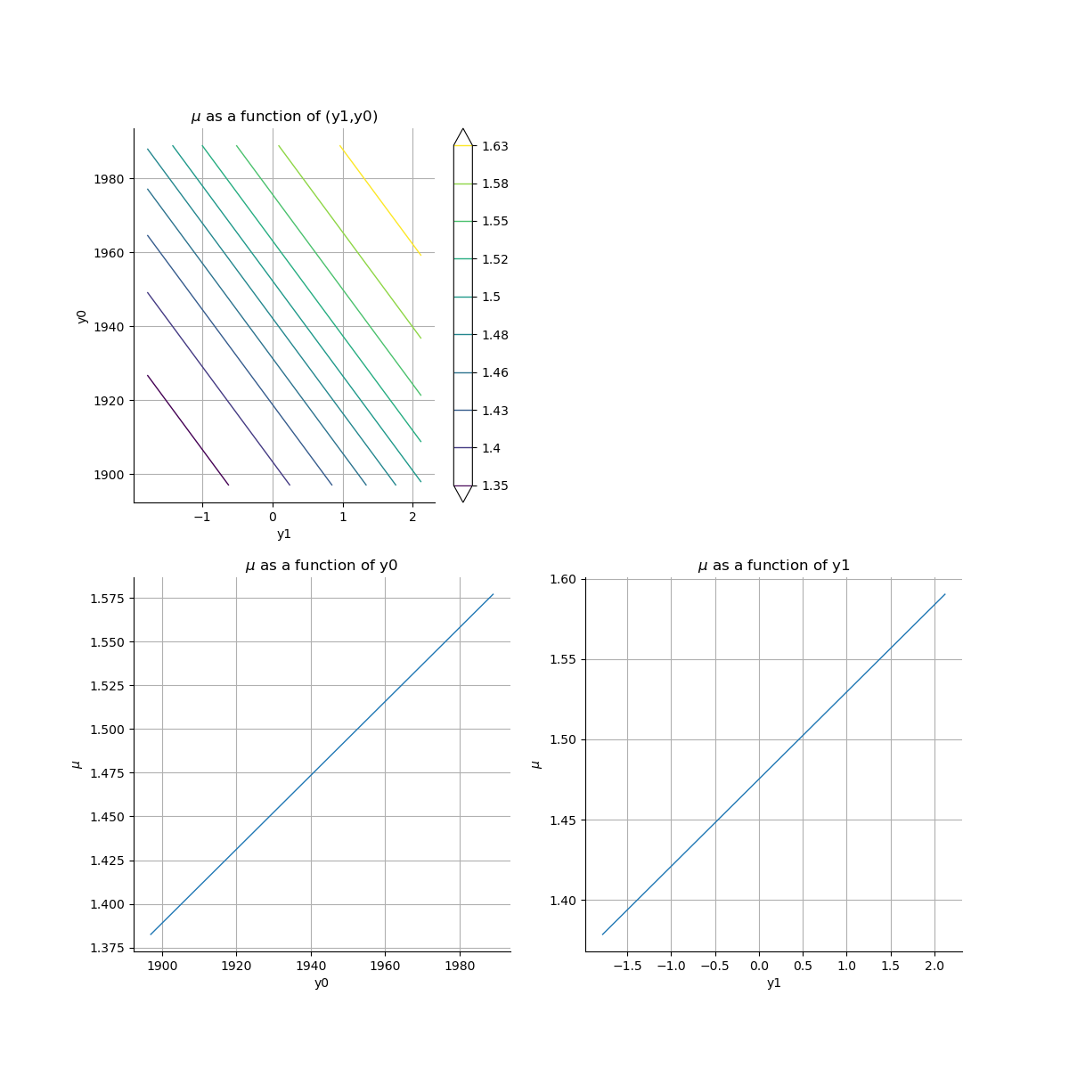
As the relation is linear (the link function is the Identity function), we get some straight lines. The third graph is the dependence on the third covariate which is constant.

refSOI = dataCovariates.computeMean()[1]
refTime = 1940
refPoint = [refTime, refSOI, 1]
gridMu = result_Cov.drawParameterFunction1D(0, refPoint)
view = otv.View(gridMu)

$, $\mu$ as a function of y0, $\mu$ as a function of y1, $\mu$ as a function of y2$

To adapt the labels and get rid of the last graph:

graphCol = gridMu.getGraphCollection()
graphMu1 = graphCol[0]
graphMu1.setTitle(r"$t \mapsto \mu(t, SOI_0)$, $SOI_0$ = {0:.2f}".format(refSOI))
graphMu1.setXTitle("t")
graphMu2 = graphCol[1]
graphMu2.setTitle(r"$SOI \mapsto \mu(t_0, SOI)$, $t_0 = $" + str(refTime))
graphMu2.setXTitle("SOI")
newGridLayout = ot.GridLayout(1, 2)
newGridLayout.setGraph(0, 0, graphMu1)
newGridLayout.setGraph(0, 1, graphMu2)
view = otv.View(newGridLayout)

$, $t \mapsto \mu(t, SOI_0)$, $SOI_0$ = -0.03, $SOI \mapsto \mu(t_0, SOI)$, $t_0 = $1940$

We plot here the graph $(t, SOI) \mapsto \mu(t, SOI)$ . As the third covariate is constant, the other graphs $(t, 1) \mapsto \mu(t, \mbox{SOI}_0, 1)$ and $(1, SOI) \mapsto \mu(t_0, 1, SOI)$ are not interesting as we have already obtained them with the previous method.

graphCol = result_Cov.drawParameterFunction2D(0, refPoint)
view = otv.View(graphCol)

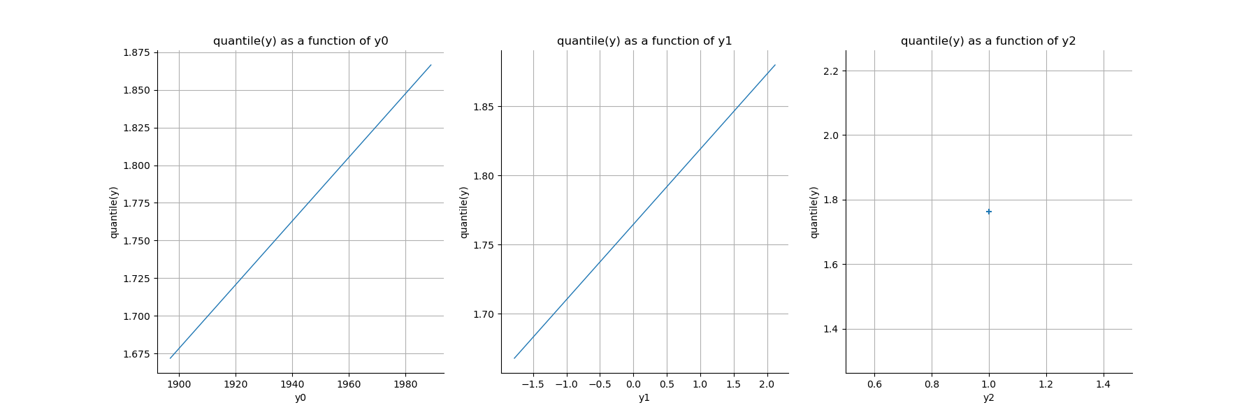
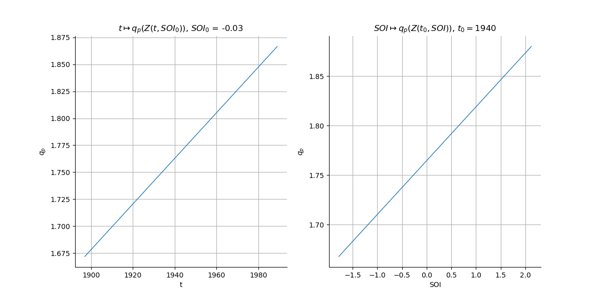
$, $\mu$ as a function of (y1,y0), $\mu$ as a function of y0, $\mu$ as a function of y1$

We plot here the graphs $t \mapsto q_p(Z_{t, \mbox{SOI}_0})$ and $\mbox{SOI} \mapsto q_p(Z_{t_0, \mbox{SOI}})$ where $Z_{t, \mbox{SOI}_0}$ is the process whose excesses of $u$ follow the estimated GPD, depending on the covariates $(t, SOI)$ . Then $q_p$ is the quantile of order $p$ . Because of the constant third covariate, the last graph is reduced to a point.

p = 0.95
gridQuantile = result_Cov.drawQuantileFunction1D(p, refPoint)
view = otv.View(gridQuantile)

, quantile(y) as a function of y0, quantile(y) as a function of y1, quantile(y) as a function of y2

To adapt the labels and get rid of the last graph:

graphCol = gridQuantile.getGraphCollection()
graphQuant1 = graphCol[0]
graphQuant1.setTitle(r"$t \mapsto q_p(Z(t, SOI_0))$, $SOI_0$ = {0:.2f}".format(refSOI))
graphQuant1.setXTitle("t")
graphQuant1.setYTitle(r"$q_p$")
graphQuant2 = graphCol[1]
graphQuant2.setTitle(r"$SOI \mapsto q_p(Z(t_0, SOI))$, $t_0 = $" + str(refTime))
graphQuant2.setXTitle("SOI")
graphQuant2.setYTitle(r"$q_p$")
newGridLayout = ot.GridLayout(1, 2)
newGridLayout.setGraph(0, 0, graphQuant1)
newGridLayout.setGraph(0, 1, graphQuant2)
view = otv.View(newGridLayout)

$, $t \mapsto q_p(Z(t, SOI_0))$, $SOI_0$ = -0.03, $SOI \mapsto q_p(Z(t_0, SOI))$, $t_0 = $1940$

otv.View.ShowAll()

Total running time of the script: (0 minutes 3.540 seconds)

OpenTURNS

An Open source initiative for the Treatment of Uncertainties, Risks'N Statistics

Previous topic

Next topic

This Page

Estimate a GEV on the Fremantle sea-levels data¶