Note

Go to the end to download the full example code.

Estimate a GEV on race times data¶

In this example, we illustrate various techniques of extreme value modeling applied to the fatest annual race times for the women’s 1500 meter event over the period 1975-1992. Readers should refer to [coles2001] to get more details.

We illustrate techniques to:

estimate a stationary and a non stationary GEV,
estimate a return level,

using:

the log-likelihood function,
the profile log-likelihood function.

This analyse is particular as we are interested in modeling the annual minimum race times and not the annual maximum race times. In order to transform the minimum modeling into a maximum modeling, we proceeds as follows.

We denote by $\tilde{M}_n = \min (X_1, \dots, X_n)$ where all the $X_i$ are independent and identically distributed variables. We introduce $Y_i = -X_i$ for $1 \leq i \leq n$ , and $M_n = \min (Y_1, \dots, Y_n)$ . Then, we have:

$\tilde{M}_n = - M_n.$

We can show that if the renormalized maximum $\tilde{M}_n$ tends to the GEV distribution parametrized by $(\mu, \sigma, \xi)$ , then the renormalized minimum $\tilde{M}_n$ tends to the GEV for minima distribution parametrized by $(\tilde{\mu}, \tilde{\sigma}, \tilde{\xi})$ where:

$\begin{align*} \tilde{\mu} & = -\mu \\ \tilde{\sigma} & = \sigma\\ \tilde{\xi} & = \xi \end{align*}$

The cumulated distribution function of $\tilde{M}_n$ , denoted by $\tilde{G}$ , is defined by:

$\tilde{G}(z) = 1-G(-z) = 1-\exp \left( -\left[ 1-\tilde{\xi} \left( \dfrac{z-\tilde{\mu}}{\tilde{\sigma}}\right)\right]^{-1/\tilde{\xi}}\right)$

for all $z$ such that $1-\tilde{\xi}(z-\tilde{\mu})/\tilde{\sigma} > 0$ .

In that example, we model the $M_n$ variable which is the annual maximum of the opposite race times.

First, we load the race times dataset. We start by looking at them through time.

import openturns as ot
import openturns.viewer as otv
from openturns.usecases import coles

data = coles.Coles().racetime
print(data[:5])

graph = ot.Graph(
    "Fastest annual women's 1500m race times", "year", "race time (s)", True, ""
)
cloud = ot.Cloud(data[:, :2])
cloud.setColor("red")
graph.add(cloud)
graph.setIntegerXTick(True)
view = otv.View(graph)

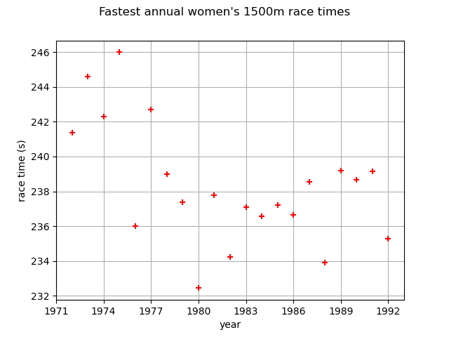
    [ Year      Race time ]
: [ 1972       241.371  ]
: [ 1973       244.616  ]
: [ 1974       242.301  ]
: [ 1975       246      ]
: [ 1976       235.994  ]

We select the race times column. We transform them into their opposite values.

sample = -1.0 * data[:, 1]

Stationary GEV modeling via the log-likelihood function

We first assume that the dependence through time is negligible, so we first model the data as independent observations over the observation period. We estimate the parameters of the GEV distribution by maximizing the log-likelihood of the data.

factory = ot.GeneralizedExtremeValueFactory()
result_LL = factory.buildMethodOfLikelihoodMaximizationEstimator(sample)

We get the fitted GEV for the variable $M_n$ and its parameters $(\hat{\mu}, \hat{\sigma}, \hat{\xi})$ .

fitted_GEV = result_LL.getDistribution()
desc = fitted_GEV.getParameterDescription()
param = fitted_GEV.getParameter()
print(", ".join([f"{p}: {value:.3f}" for p, value in zip(desc, param)]))

mu: -239.260, sigma: 3.643, xi: -0.470

We get the asymptotic distribution of the estimator $(\hat{\mu}, \hat{\sigma}, \hat{\xi})$ . In that case, the asymptotic distribution is normal.

parameterEstimate = result_LL.getParameterDistribution()
print("Asymptotic distribution of the estimator : ")
print(parameterEstimate)

Asymptotic distribution of the estimator :
Normal(mu = [-239.26,3.64268,-0.469834], sigma = [0.891274,0.778059,0.236181], R = [[  1        -0.113124 -0.406653 ]
 [ -0.113124  1        -0.706993 ]
 [ -0.406653 -0.706993  1        ]])

We get the covariance matrix and the standard deviation of $(\hat{\mu}, \hat{\sigma}, \hat{\xi})$ .

print("Cov matrix = \n", parameterEstimate.getCovariance())
print("Standard dev = ", parameterEstimate.getStandardDeviation())

Cov matrix =
 [[  0.79437   -0.0784475 -0.0856013 ]
 [ -0.0784475  0.605376  -0.129919  ]
 [ -0.0856013 -0.129919   0.0557815 ]]
Standard dev =  [0.891274,0.778059,0.236181]

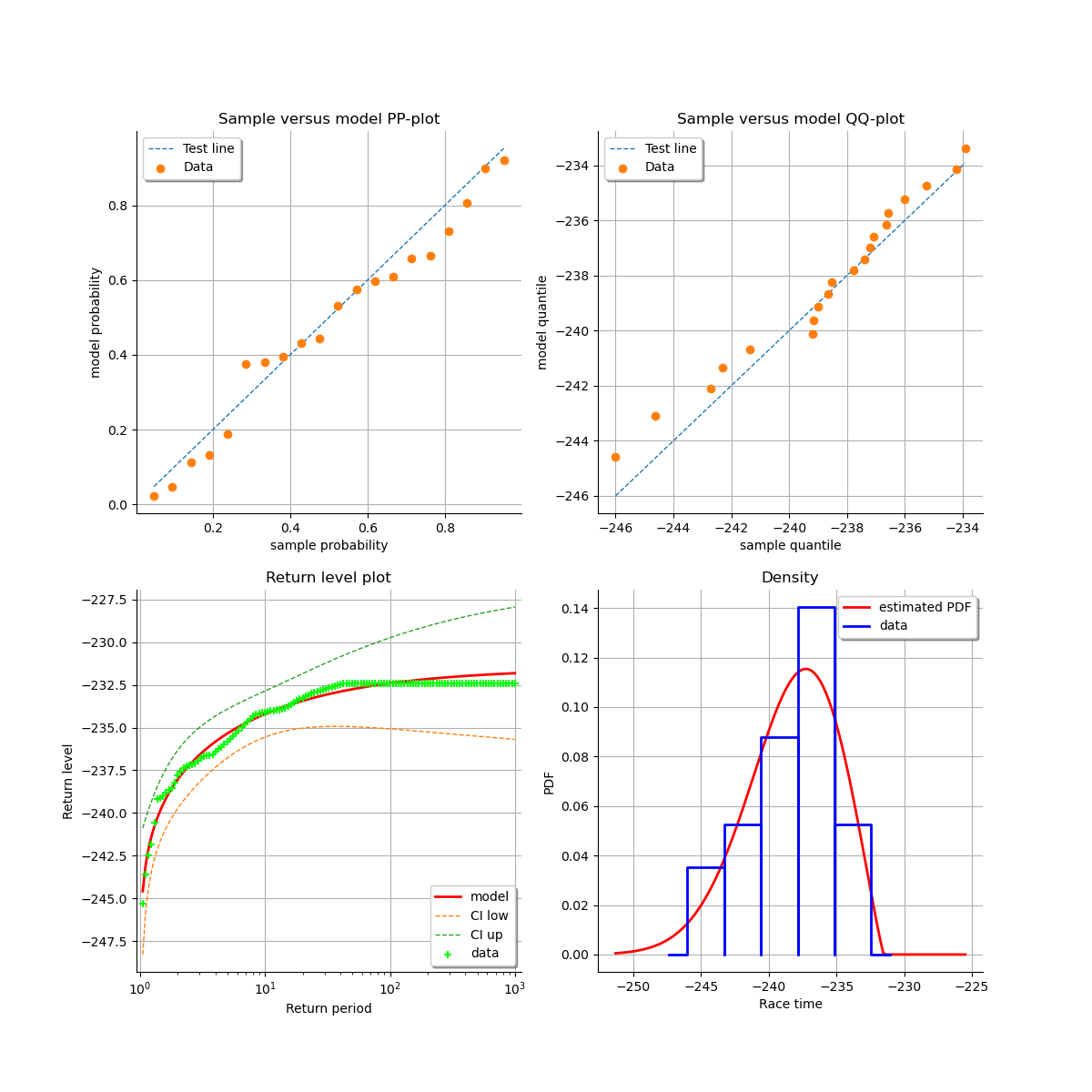
At last, we can validate the inference result thanks the 4 usual diagnostic plots:

the probability-probability pot,
the quantile-quantile pot,
the return level plot,
the data histogram and the density of the fitted model.

validation = ot.GeneralizedExtremeValueValidation(result_LL, sample)
graph = validation.drawDiagnosticPlot()
view = otv.View(graph)

, Sample versus model PP-plot, Sample versus model QQ-plot, Return level plot, Density

Stationary GEV modeling via the profile log-likelihood function

Now, we use the profile log-likehood function rather than log-likehood function to estimate the parameters of the GEV.

result_PLL = factory.buildMethodOfXiProfileLikelihoodEstimator(sample)

The following graph allows one to get the profile log-likelihood plot. It also indicates the optimal value of $\xi$ , the maximum profile log-likelihood and the confidence interval for $\xi$ of order 0.95 (which is the default value).

order = 0.95
result_PLL.setConfidenceLevel(order)
view = otv.View(result_PLL.drawProfileLikelihoodFunction())

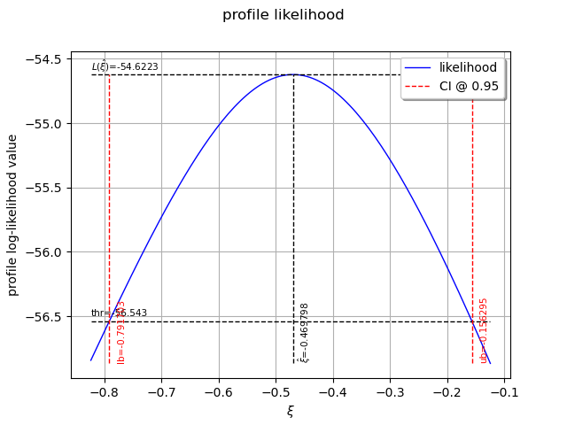
We can get the numerical values of the confidence interval: it appears to be a bit smaller with the interval obtained from the profile log-likelihood function than with the log-likelihood function. Note that if the order requested is too high, the confidence interval might not be calculated because one of its bound is out of the definition domain of the log-likelihood function.

try:
    print("Confidence interval for xi = ", result_PLL.getParameterConfidenceInterval())
except Exception as ex:
    print(type(ex))
    pass

Confidence interval for xi =  [-0.791703, -0.156295]

Return level estimate from the estimated stationary GEV

We estimate the $m$ -block return level $z_m$ : it is computed as a particular quantile of the GEV model estimated using the log-likelihood function. We just have to use the maximum log-likelihood estimator built in the previous section. The return level of $M_n$ and $\tilde{M}_n$ have opposite values.

As the data are annual sea-levels, each block corresponds to one year: the 10-year return level corresponds to $m=10$ and the 100-year return level corresponds to $m=100$ .

The method provides the asymptotic distribution of the estimator $\hat{z}_m$ of $M_n$ which mean is the return-level estimate.

zm_10 = factory.buildReturnLevelEstimator(result_LL, 10.0)
return_level_10 = zm_10.getMean()
print("Maximum log-likelihood function : ")
print(f"10-year return level={return_level_10}")
return_level_ci10 = zm_10.computeBilateralConfidenceInterval(0.95)
print(f"CI={return_level_ci10}")

Maximum log-likelihood function :
10-year return level=[-234.2]
CI=[-235.552, -232.849]

zm_100 = factory.buildReturnLevelEstimator(result_LL, 100.0)
return_level_100 = zm_100.getMean()
print(f"100-year return level={return_level_100}")
return_level_ci100 = zm_100.computeBilateralConfidenceInterval(0.95)
print(f"CI={return_level_ci100}")

100-year return level=[-232.4]
CI=[-235.071, -229.729]

Return level estimate via the profile log-likelihood function of a stationary GEV

We can estimate the $m$ -block return level $z_m$ directly from the data using the profile likelihood with respect to $z_m$ .

result_zm_10_PLL = factory.buildReturnLevelProfileLikelihoodEstimator(sample, 10.0)
zm_10_PLL = result_zm_10_PLL.getParameter()
print(f"10 years return level (profile)={zm_10_PLL}")

10 years return level (profile)=-234.20091228177077

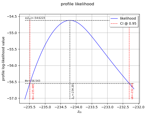
We can get the confidence interval of $z_m$ : once more, it appears to be a bit smaller than the interval obtained from the log-likelihood function. As for the confidence interval of $\xi$ , dependeding on the order requested, the interval might not be calculated.

result_zm_10_PLL.setConfidenceLevel(0.95)
try:
    return_level_ci10 = result_zm_10_PLL.getParameterConfidenceInterval()
except Exception as ex:
    print(type(ex))
    pass
print("Maximum profile log-likelihood function : ")
print(f"CI={return_level_ci10}")

Maximum profile log-likelihood function :
CI=[-235.485, -232.301]

We can also plot the profile log-likelihood function and get the confidence interval, the optimal value of $z_m$ and its confidence interval.

view = otv.View(result_zm_10_PLL.drawProfileLikelihoodFunction())

Non stationary GEV modeling via the log-likelihood function

If we look at the data carefully, we see that the pattern of variation has not remained constant over the observation period. There is an increase in the data through time. We want to model this trend because a slight increase in extreme sea-levels might have a significant impact on the safety of coastal flood defenses.

We still work on the $M_n$ variable. First we need to get the time stamps (in years here).

timeStamps = data[:, 0]

Then, we define the functional basis for each parameter of the GEV model. Even if we have the possibility to affect a time-varying model to each of the 3 parameters $(\mu, \sigma, \xi)$ , it is strongly recommended not to vary the parameter $\xi$ and to let it constant.

For numerical reasons, it is strongly recommended to normalize all the data as follows:

$\tau(t) = \dfrac{t-c}{d}$

where:

the CenterReduce method where $c = \dfrac{1}{n} \sum_{i=1}^n t_i$ is the mean time stamps and $d = \sqrt{\dfrac{1}{n} \sum_{i=1}^n (t_i-c)^2}$ is the standard deviation of the time stamps;
the MinMax method where $c = t_1$ is the initial time and $d = t_n-t_1$ the final time;
the None method where $c = 0$ and $d = 1$ : in that case, data are not normalized.

We suppose that $\mu$ is linear in time, and that the other parameters remain constant.

$\begin{align*} \mu(t) & = \beta_1 + \beta_2\tau(t) \\ \sigma(t) & = \beta_3 \\ \xi(t) & = \beta_4 \end{align*}$

constant = ot.SymbolicFunction(["t"], ["1.0"])
basis = ot.Basis([constant, ot.SymbolicFunction(["t"], ["t"])])
# basis for mu, sigma, xi
muIndices = [0, 1]  # linear
sigmaIndices = [0]  # stationary
xiIndices = [0]  # stationary

We can now estimate the list of coefficients $\vect{\beta} = (\beta_1, \beta_2, \beta_3, \beta_4)$ using the log-likelihood of the data. We test the 3 normalizing methods and both initial points in order to evaluate their impact on the results. We can see that:

both normalization methods lead to the same result for $\beta_1$ , $\beta_3$ and $\beta_4$ (note that $\beta_2$ depends on the normalization function),
both initial points lead to the same result when the data have been normalized,
it is very important to normalize all the data: if not, the result strongly depends on the initial point and it differs from the result obtained with normalized data. The results are not optimal in that case since the associated log-likelihood are much smaller than those obtained with normalized data.

ot.ResourceMap.SetAsUnsignedInteger(
    "GeneralizedExtremeValueFactory-MaximumCallsNumber", 1000000
)
print("Linear mu(t) model: ")
for normMeth in ["MinMax", "CenterReduce", "None"]:
    for initPoint in ["Gumbel", "Static"]:
        print(f"normMeth = {normMeth}, initPoint = {initPoint}")
        # The ot.Function() is the identity function.
        result = factory.buildTimeVarying(
            sample,
            timeStamps,
            basis,
            muIndices,
            sigmaIndices,
            xiIndices,
            ot.Function(),
            ot.Function(),
            ot.Function(),
            initPoint,
            normMeth,
        )
        beta = result.getOptimalParameter()
        print(f"beta = {beta}")
        print(f"Max log-likelihood = {result.getLogLikelihood()}")

Linear mu(t) model:
normMeth = MinMax, initPoint = Gumbel
beta = [-242.635,6.25776,2.73173,-0.201353]
Max log-likelihood = -51.894041784037256
normMeth = MinMax, initPoint = Static
beta = [-242.635,6.25761,2.73174,-0.201365]
Max log-likelihood = -51.89404185837069
normMeth = CenterReduce, initPoint = Gumbel
beta = [-239.506,1.94196,2.73164,-0.201298]
Max log-likelihood = -51.89404130255576
normMeth = CenterReduce, initPoint = Static
beta = [-239.506,1.94201,2.73163,-0.201294]
Max log-likelihood = -51.894041292150014
normMeth = None, initPoint = Gumbel
beta = [-239.942,-0.000578171,2.80599,0.0958746]
Max log-likelihood = -61.18805537945545
normMeth = None, initPoint = Static
beta = [-239.26,1.15331e-06,3.6427,-0.469838]
Max log-likelihood = -54.622262531545104

According to the previous results, we choose the MinMax normalization method and the Gumbel initial point. This initial point is cheaper than the Static one as it requires no optimization computation.

result_NonStatLL = factory.buildTimeVarying(
    sample,
    timeStamps,
    basis,
    muIndices,
    sigmaIndices,
    xiIndices,
    ot.Function(),
    ot.Function(),
    ot.Function(),
    "Gumbel",
    "MinMax",
)
beta = result_NonStatLL.getOptimalParameter()
print("Linear mu(t) model : ")
print(f"beta = {beta}")
print(f"mu(t) = {beta[0]:.4f} + {beta[1]:.4f} * tau")
print(f"sigma = = {beta[2]:.4f}")
print(f"xi = = {beta[3]:.4f}")

Linear mu(t) model :
beta = [-242.635,6.25776,2.73173,-0.201353]
mu(t) = -242.6347 + 6.2578 * tau
sigma = = 2.7317
xi = = -0.2014

You can get the expression of the normalizing function $t \mapsto \tau(t)$ :

normFunc = result_NonStatLL.getNormalizationFunction()
print("Function tau(t): ", normFunc)
print("c = ", normFunc.getEvaluation().getImplementation().getCenter()[0])
print("1/d = ", normFunc.getEvaluation().getImplementation().getLinear()[0, 0])

Function tau(t):  class=LinearFunction name=Unnamed implementation=class=LinearEvaluation name=Unnamed center=[1972] constant=[0] linear=[[ 0.05 ]]
c =  1972.0
1/d =  0.05

You can get the function $t \mapsto \vect{\theta}(t)$ where $\vect{\theta}(t) = (\mu(t), \sigma(t), \xi(t))$ .

functionTheta = result_NonStatLL.getParameterFunction()

We get the asymptotic distribution of $\vect{\beta}$ to compute some confidence intervals of the estimates, for example of order $p = 0.95$ .

dist_beta = result_NonStatLL.getParameterDistribution()
confidence_level = 0.95
for i in range(beta.getSize()):
    lower_bound = dist_beta.getMarginal(i).computeQuantile((1 - confidence_level) / 2)[
        0
    ]
    upper_bound = dist_beta.getMarginal(i).computeQuantile((1 + confidence_level) / 2)[
        0
    ]
    print(
        "Conf interval for beta_"
        + str(i + 1)
        + " = ["
        + str(lower_bound)
        + "; "
        + str(upper_bound)
        + "]"
    )

Conf interval for beta_1 = [-243.1574557477432; -242.11202993332392]
Conf interval for beta_2 = [5.216499414292534; 7.299026584173018]
Conf interval for beta_3 = [2.456616349866622; 3.006835164775891]
Conf interval for beta_4 = [-0.3126093022867582; -0.09009579763055493]

In order to compare different modelings, we get the optimal log-likelihood of the data for both stationary and non stationary models. The difference is significant enough to be in favor of the non stationary model.

print("Max log-likelihood: ")
print("Stationary model =  ", result_LL.getLogLikelihood())
print("Non stationary linear mu(t) model =  ", result_NonStatLL.getLogLikelihood())

Max log-likelihood:
Stationary model =   -54.622265554594776
Non stationary linear mu(t) model =   -51.894041784037256

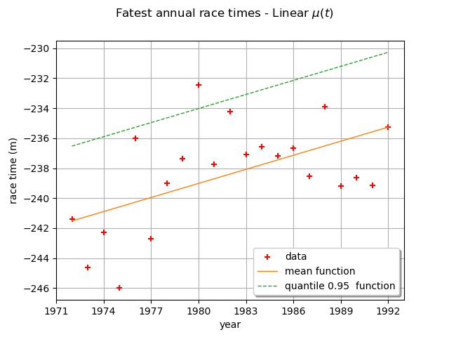
We can draw the mean function $t \mapsto \Expect{\mbox{GEV}(t)}$ . Be careful, it is not the function $t \mapsto \mu(t)$ . As a matter of fact, the mean is defined for $\xi <1$ only and in that case, for $\xi \neq 0$ , we have:

$\Expect{\mbox{GEV}(t)} = \mu(t) + \dfrac{\sigma(t)}{\xi(t)} (\Gamma(1-\xi(t))-1)$

and for $\xi = 0$ , we have:

$\Expect{\mbox{GEV}(t)} = \mu(t) + \sigma(t)\gamma$

where $\gamma$ is the Euler constant.

We can also draw the function $t \mapsto q_p(t)$ where $q_p(t)$ is the quantile of order $p$ of the GEV distribution at time $t$ . Here, $\mu(t)$ is a linear function and the other parameters are constant, so the mean and the quantile functions are also linear functions.

The graph confirms the increase of the annual maximum sea-levels through time.

graph = ot.Graph(
    r"Fatest annual race times - Linear $\mu(t)$", "year", "race time (m)", True, ""
)
dataModified = data * ot.Point([1.0, -1.0])
graph.setIntegerXTick(True)
# data
cloud = ot.Cloud(dataModified)
cloud.setColor("red")
graph.add(cloud)
# mean function
meandata = [
    result_NonStatLL.getDistribution(t).getMean()[0] for t in data[:, 0].asPoint()
]
curve_meanPoints = ot.Curve(data[:, 0].asPoint(), meandata)
graph.add(curve_meanPoints)
# quantile function
graphQuantile = result_NonStatLL.drawQuantileFunction(0.95)
drawQuant = graphQuantile.getDrawable(0)
drawQuant = graphQuantile.getDrawable(0)
drawQuant.setLineStyle("dashed")
graph.add(drawQuant)
graph.setLegends(["data", "mean function", "quantile 0.95  function"])
graph.setLegendPosition("lower right")
view = otv.View(graph)

$Fatest annual race times - Linear $\mu(t)$$

At last, we can test the validity of the stationary model $\mathcal{M}_0$ relative to the model with time varying parameters $\mathcal{M}_1$ . The model $\mathcal{M}_0$ is parametrized by $(\beta_1, \beta_3, \beta_4)$ and the model $\mathcal{M}_1$ is parametrized by $(\beta_1, \beta_2, \beta_3, \beta_4)$ : so we have $\mathcal{M}_0 \subset \mathcal{M}_1$ .

We use the Likelihood Ratio test. The null hypothesis is the stationary model $\mathcal{M}_0$ . The Type I error $\alpha$ is taken equal to 0.05.

This test confirms that the dependence through time is not negligible: it means that the linear model:math:mu(t) component explains a large variation in the data.

llh_LL = result_LL.getLogLikelihood()
llh_NonStatLL = result_NonStatLL.getLogLikelihood()
modelM0_Nb_param = 3
modelM1_Nb_param = 4
resultLikRatioTest = ot.HypothesisTest.LikelihoodRatioTest(
    modelM0_Nb_param, llh_LL, modelM1_Nb_param, llh_NonStatLL, 0.05
)
accepted = resultLikRatioTest.getBinaryQualityMeasure()
print(
    f"Hypothesis H0 (stationary model) vs  H1 (linear mu(t) model):  accepted ? = {accepted}"
)

Hypothesis H0 (stationary model) vs  H1 (linear mu(t) model):  accepted ? = False

We detail the statistics of the Likelihood Ratio test: the deviance statistics $\mathcal{D}_p$ follows a $\chi^2_1$ distribution. The model $\mathcal{M}_0$ is rejected if the deviance statistics estimated on the data is greater than the threshold $c_{\alpha}$ or if the p-value is less than the Type I error $\alpha = 0.05$ .

print(f"Dp={resultLikRatioTest.getStatistic():.2f}")
print(f"alpha={resultLikRatioTest.getThreshold():.2f}")
print(f"p-value={resultLikRatioTest.getPValue():.2f}")

Dp=5.46
alpha=0.05
p-value=0.02

We can perform the same study with a quadratic model for $\mu(t)$ :

$\begin{align*} \mu(t) & = \beta_1 + \beta_2 \tau(t) + \beta_3\tau(t)^2 \\ \sigma(t) & = \beta_4 \\ \xi(t) & = \beta_5 \end{align*}$

basis = ot.Basis(
    [constant, ot.SymbolicFunction(["t"], ["t"]), ot.SymbolicFunction(["t"], ["t^2"])]
)
result_NonStatLL_2 = factory.buildTimeVarying(
    sample,
    timeStamps,
    basis,
    [0, 1, 2],
    [0],
    [0],
    ot.Function(),
    ot.Function(),
    ot.Function(),
    "Gumbel",
    "MinMax",
)
beta = result_NonStatLL_2.getOptimalParameter()
print("Quadratic mu(t) model : ")
print("beta1, beta2, beta3, beta4, beta5 = ", beta)
print(f"mu(t) = {beta[0]:.4f} + {beta[1]:.4f} * tau + {beta[2]:.4f} * tau^2")
print(f"sigma = {beta[3]:.4f}")
print(f"xi = {beta[4]:.4f}")

Quadratic mu(t) model :
beta1, beta2, beta3, beta4, beta5 =  [-243.454,13.2016,-7.37734,2.5237,-0.221073]
mu(t) = -243.4542 + 13.2016 * tau + -7.3773 * tau^2
sigma = 2.5237
xi = -0.2211

We get the asymptotic distribution of $\vect{\beta}$ to compute some confidence intervals of the estimates, for example of order $p = 0.95$ .

dist_beta = result_NonStatLL_2.getParameterDistribution()
confidence_level = 0.95
for i in range(beta.getSize()):
    lower_bound = dist_beta.getMarginal(i).computeQuantile((1 - confidence_level) / 2)[
        0
    ]
    upper_bound = dist_beta.getMarginal(i).computeQuantile((1 + confidence_level) / 2)[
        0
    ]
    print(
        "Conf interval for beta_"
        + str(i + 1)
        + " = ["
        + str(lower_bound)
        + "; "
        + str(upper_bound)
        + "]"
    )

Conf interval for beta_1 = [-244.287417882467; -242.62107538432625]
Conf interval for beta_2 = [8.497738808703389; 17.90540730309058]
Conf interval for beta_3 = [-11.974692053671532; -2.7799858455459985]
Conf interval for beta_4 = [2.287755446156212; 2.7596448403596714]
Conf interval for beta_5 = [-0.3298681130077343; -0.11227714586730275]

In order to compare different modelings, we get the optimal log-likelihood of the data for both stationary and non stationary models. The difference is significant enough to be in favor of the non stationary model.

print("Max log-likelihood = ")
print("Non stationary quadratic mu(t) model = ", result_NonStatLL_2.getLogLikelihood())

Max log-likelihood =
Non stationary quadratic mu(t) model =  -49.95079559010807

At last, we can test the validity of the non stationary model $\mathcal{M}_0$ where $\mu(t)$ is linear relative to the model $\mathcal{M}_1$ where $\mu(t)$ is quadratic. The model $\mathcal{M}_0$ is parametrized by $(\beta_1, \beta_2, \beta_3, \beta_4)$ and the model $\mathcal{M}_1$ is parametrized by $(\beta_1, \beta_2, \beta_3, \beta_4, \beta_5)$ : so we have $\mathcal{M}_0 \subset \mathcal{M}_1$ .

We use the Likelihood Ratio test. The null hypothesis is the stationary model $\mathcal{M}_0$ . The Type I error $\alpha$ is taken equal to 0.05.

This test confirms that the dependence through time is not negligible: it means that the $\mu(t)$ quadratic model explains even better a large variation in the data.

llh_NonStatLL_2 = result_NonStatLL_2.getLogLikelihood()
resultLikRatioTest = ot.HypothesisTest.LikelihoodRatioTest(
    4, llh_NonStatLL, 5, llh_NonStatLL_2, 0.05
)
accepted = resultLikRatioTest.getBinaryQualityMeasure()
print(
    f"Hypothesis H0 (linear mu(t) model) vs H1 (quadratic mu(t) model):  accepted ? = {accepted}"
)

Hypothesis H0 (linear mu(t) model) vs H1 (quadratic mu(t) model):  accepted ? = False

otv.View.ShowAll()

Total running time of the script: (0 minutes 2.096 seconds)

OpenTURNS

An Open source initiative for the Treatment of Uncertainties, Risks'N Statistics

Previous topic

Next topic

This Page

Estimate a GEV on race times data¶