Note

Go to the end to download the full example code.

Kriging: choose a polynomial trend¶

import openturns as ot
import openturns.viewer as otv
from matplotlib import pylab as plt

Introduction¶

In this example we present the polynomial trends which we may use in a Kriging metamodel. This example focuses on three polynomial trends:

In the Kriging: choose a polynomial trend on the beam model example, we give another example of this method. In the Kriging: choose an arbitrary trend example, we show how to configure an arbitrary trend.

The model is the real function:

$\model(x) = x \sin \left( \frac{x}{2} \right)$

for any $x \in [0,10]$ . We consider the MaternModel covariance kernel where $\vect{\theta} = (\sigma, \rho)$ is the vector of hyperparameters. The covariance model is fixed but its parameters must be calibrated depending on the data. The Kriging metamodel is:

$\widehat{Y}(x) = m(x) + Z(x)$

where $m(.)$ is the trend and $Z(.)$ is a Gaussian process with zero mean and covariance model $C_{\vect{\theta}}(s,t)$ . The trend is deterministic and the Gaussian process is probabilistic but they both contribute to the metamodel. A special feature of the Kriging is the interpolation property: the metamodel is exact at the training data.

covarianceModel = ot.SquaredExponential([1.0], [1.0])

Define the model¶

First, we define the MaternModel covariance model.

covarianceModel = ot.MaternModel([1.0], [1.0], 2.5)

We define our exact model with a SymbolicFunction.

model = ot.SymbolicFunction(["x"], ["x * sin(0.5 * x)"])

We use the following sample to train our metamodel.

xmin = 0.0
xmax = 10.0
ot.RandomGenerator.SetSeed(0)
nTrain = 8
Xtrain = ot.Uniform(xmin, xmax).getSample(nTrain).sort()
Xtrain

	v0
0	0.3250275
1	1.352764
2	3.47057
3	5.030402
4	6.298766
5	8.828052
6	9.206796
7	9.69423

The values of the exact model are also needed for training.

Ytrain = model(Xtrain)
Ytrain

	y0
0	0.05258924
1	0.8467968
2	3.423725
3	2.94895
4	-0.0490677
5	-8.43802
6	-9.152166
7	-9.606383

We shall test the model on a set of points based on a regular grid.

nTest = 100
step = (xmax - xmin) / (nTest - 1)
x_test = ot.RegularGrid(xmin, step, nTest).getVertices()

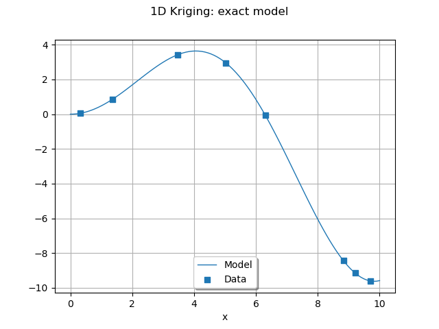
We draw the training points and the model at the testing points. We encapsulate it into a function to use it again later.

def plot_exact_model(color):
    graph = ot.Graph("", "x", "", True, "")
    y_test = model(x_test)
    curveModel = ot.Curve(x_test, y_test)
    curveModel.setLineStyle("solid")
    curveModel.setColor(color)
    curveModel.setLegend("Model")
    graph.add(curveModel)
    cloud = ot.Cloud(Xtrain, Ytrain)
    cloud.setColor(color)
    cloud.setPointStyle("fsquare")
    cloud.setLegend("Data")
    graph.add(cloud)
    graph.setLegendPosition("bottom")
    return graph

palette = ot.Drawable.BuildDefaultPalette(5)
graph = plot_exact_model(palette[0])
graph.setTitle("1D Kriging: exact model")
view = otv.View(graph)

Scale the input training sample¶

We often have to apply a transform on the input data before performing the Kriging. This make the estimation of the hyperparameters of the Kriging metamodel easier for the optimization algorithm. To do so we write a linear transform of our input data: we make it unit centered at its mean. Then we fix the mean and the standard deviation to their values with the ParametricFunction. We build the inverse transform as well.

We first compute the mean and standard deviation of the input data.

mean = Xtrain.computeMean()[0]
stdDev = Xtrain.computeStandardDeviation()[0]
print("Xtrain, mean: %.3f" % mean)
print("Xtrain, standard deviation: %.3f" % stdDev)

Xtrain, mean: 5.526
Xtrain, standard deviation: 3.613

tf = ot.SymbolicFunction(["mu", "sigma", "x"], ["(x - mu) / sigma"])
itf = ot.SymbolicFunction(["mu", "sigma", "x"], ["sigma * x + mu"])
myInverseTransform = ot.ParametricFunction(itf, [0, 1], [mean, stdDev])
myTransform = ot.ParametricFunction(tf, [0, 1], [mean, stdDev])

Scale the input training sample.

scaledXtrain = myTransform(Xtrain)
scaledXtrain

	y0
0	-1.439601
1	-1.15512
2	-0.5689025
3	-0.1371353
4	0.2139527
5	0.9140688
6	1.018907
7	1.15383

Constant basis¶

In this paragraph we choose a basis constant for the Kriging. This trend only has one parameter which is the value of the constant. The basis is built with the ConstantBasisFactory class.

dimension = 1
basis = ot.ConstantBasisFactory(dimension).build()

We build the Kriging algorithm by giving it the transformed data, the output data, the covariance model and the basis.

algo = ot.KrigingAlgorithm(scaledXtrain, Ytrain, covarianceModel, basis)

We can run the algorithm and store the result.

algo.run()
result = algo.getResult()

The metamodel is the following ComposedFunction.

metamodel = ot.ComposedFunction(result.getMetaModel(), myTransform)

Define a function to plot the metamodel

def plotMetamodel(x_test, krigingResult, myTransform, color):
    scaled_x_test = myTransform(x_test)
    metamodel = result.getMetaModel()
    y_test = metamodel(scaled_x_test)
    curve = ot.Curve(x_test, y_test)
    curve.setLineStyle("dashed")
    curve.setColor(color)
    curve.setLegend("Metamodel")
    return curve

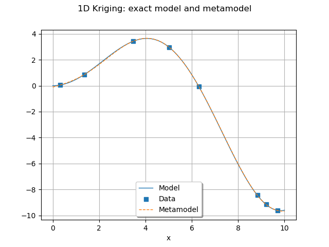
We can draw the metamodel and the exact model on the same graph.

graph = plot_exact_model(palette[0])
graph.add(plotMetamodel(x_test, result, myTransform, palette[1]))
graph.setTitle("1D Kriging: exact model and metamodel")
view = otv.View(graph)

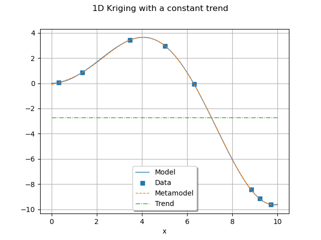
We can retrieve the calibrated trend coefficient with getTrendCoefficients().

c0 = result.getTrendCoefficients()
print("The trend is the curve m(x) = %.6e" % c0[0])

The trend is the curve m(x) = -2.726225e+00

We also observe the values of the hyperparameters of the trained covariance model.

rho = result.getCovarianceModel().getScale()[0]
print("Scale parameter: %.3e" % rho)

sigma = result.getCovarianceModel().getAmplitude()[0]
print("Amplitude parameter: %.3e" % sigma)

Scale parameter: 1.368e+00
Amplitude parameter: 6.077e+00

We build the trend from the coefficient.

constantTrend = ot.SymbolicFunction(["a", "x"], ["a"])
myTrend = ot.ParametricFunction(constantTrend, [0], [c0[0]])

Define a function to plot the trend.

def plotTrend(x_test, myTrend, myTransform, color):
    scale_x_test = myTransform(x_test)
    y_test = myTrend(scale_x_test)
    curve = ot.Curve(x_test, y_test)
    curve.setLineStyle("dotdash")
    curve.setColor(color)
    curve.setLegend("Trend")
    return curve

We draw the trend found by the Kriging procedure.

graph.add(plotTrend(x_test, myTrend, myTransform, palette[2]))
graph.setTitle("1D Kriging with a constant trend")
view = otv.View(graph)

Create a function to plot confidence bounds.

def plotKrigingConfidenceBounds(krigingResult, x_test, myTransform, color, alpha=0.05):
    bilateralCI = ot.Normal().computeBilateralConfidenceInterval(1.0 - alpha)
    quantileAlpha = bilateralCI.getUpperBound()[0]
    sqrt = ot.SymbolicFunction(["x"], ["sqrt(x)"])
    n_test = x_test.getSize()
    epsilon = ot.Sample(n_test, [1.0e-8])
    scaled_x_test = myTransform(x_test)
    conditionalVariance = (
        krigingResult.getConditionalMarginalVariance(scaled_x_test) + epsilon
    )
    conditionalSigma = sqrt(conditionalVariance)
    metamodel = krigingResult.getMetaModel()
    y_test = metamodel(scaled_x_test)
    dataLower = [
        y_test[i, 0] - quantileAlpha * conditionalSigma[i, 0] for i in range(n_test)
    ]
    dataUpper = [
        y_test[i, 0] + quantileAlpha * conditionalSigma[i, 0] for i in range(n_test)
    ]
    boundsPoly = ot.Polygon.FillBetween(x_test.asPoint(), dataLower, dataUpper)
    boundsPoly.setColor(color)
    boundsPoly.setLegend("%d%% C.I." % ((1.0 - alpha) * 100))
    return boundsPoly

Plot a confidence interval.

graph.add(plotKrigingConfidenceBounds(result, x_test, myTransform, palette[3]))
graph.setTitle("1D Kriging with a constant trend")
graph.setLegendCorner([1.0, 1.0])
graph.setLegendPosition("upper left")
view = otv.View(
    graph,
    figure_kw={"figsize": (7.0, 3.0)},
)

plt.subplots_adjust(right=0.6)

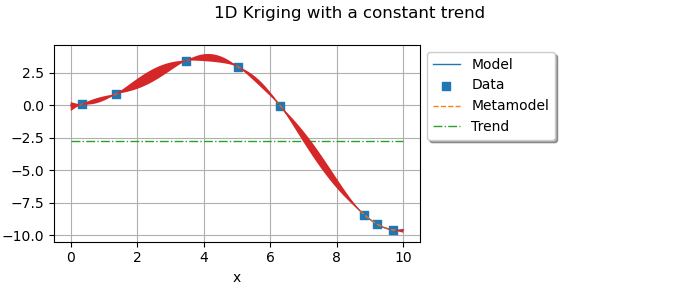
As expected with a constant basis, the trend obtained is an horizontal line.

Linear basis¶

With a linear basis, the vector space is defined by the basis $\{1, z\}$ : that is all the lines of the form $y(z) = az + b$ where $a$ and $b$ are real parameters.

basis = ot.LinearBasisFactory(dimension).build()

We run the Kriging analysis and store the result.

algo = ot.KrigingAlgorithm(scaledXtrain, Ytrain, covarianceModel, basis)
algo.run()
result = algo.getResult()
metamodel = ot.ComposedFunction(result.getMetaModel(), myTransform)

We can draw the metamodel and the exact model on the same graph.

graph = plot_exact_model(palette[0])
graph.add(plotMetamodel(x_test, result, myTransform, palette[1]))

We can retrieve the calibrated trend coefficients with getTrendCoefficients().

c0 = result.getTrendCoefficients()
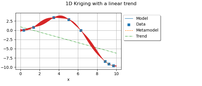
print("Trend is the curve m(X) = %.6e X + %.6e" % (c0[1], c0[0]))

Trend is the curve m(X) = -2.578407e+00 X + -3.020888e+00

We observe the values of the hyperparameters of the trained covariance model.

rho = result.getCovarianceModel().getScale()[0]
print("Scale parameter: %.3e" % rho)

sigma = result.getCovarianceModel().getAmplitude()[0]
print("Amplitude parameter: %.3e" % sigma)

Scale parameter: 1.100e+00
Amplitude parameter: 4.627e+00

We draw the linear trend that we are interested in.

linearTrend = ot.SymbolicFunction(["a", "b", "z"], ["a * z + b"])
myTrend = ot.ParametricFunction(linearTrend, [0, 1], [c0[1], c0[0]])
graph.add(plotTrend(x_test, myTrend, myTransform, palette[2]))

Add the 95% confidence interval.

graph.add(plotKrigingConfidenceBounds(result, x_test, myTransform, palette[3]))
graph.setTitle("1D Kriging with a linear trend")
graph.setLegendCorner([1.0, 1.0])
graph.setLegendPosition("upper left")
view = otv.View(
    graph,
    figure_kw={"figsize": (7.0, 3.0)},
)

plt.subplots_adjust(right=0.6)

Quadratic basis¶

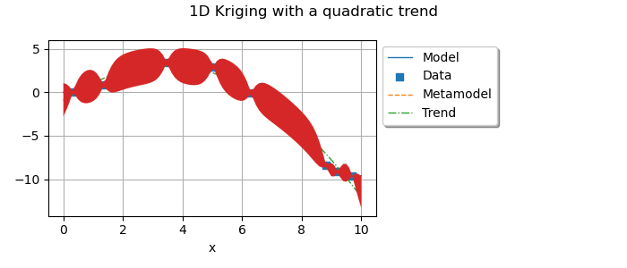
In this last paragraph we turn to the quadratic basis. All subsequent analysis should remain the same.

basis = ot.QuadraticBasisFactory(dimension).build()

We run the Kriging analysis and store the result.

algo = ot.KrigingAlgorithm(scaledXtrain, Ytrain, covarianceModel, basis)
algo.run()
result = algo.getResult()
metamodel = ot.ComposedFunction(result.getMetaModel(), myTransform)

We can draw the metamodel and the exact model on the same graph.

graph = plot_exact_model(palette[0])
graph.add(plotMetamodel(x_test, result, myTransform, palette[1]))

We can retrieve the calibrated trend coefficients with getTrendCoefficients().

c0 = result.getTrendCoefficients()
print("Trend is the curve m(X) = %.6e Z**2 + %.6e Z + %.6e" % (c0[2], c0[1], c0[0]))

Trend is the curve m(X) = -4.583776e+00 Z**2 + -5.327795e+00 Z + 1.564663e+00

We observe the values of the hyperparameters of the trained covariance model.

rho = result.getCovarianceModel().getScale()[0]
print("Scale parameter: %.3e" % rho)

sigma = result.getCovarianceModel().getAmplitude()[0]
print("Amplitude parameter: %.3e" % sigma)

Scale parameter: 8.374e-02
Amplitude parameter: 9.440e-01

The quadratic trend obtained.

quadraticTrend = ot.SymbolicFunction(["a", "b", "c", "z"], ["a * z^2 + b * z + c"])
myTrend = ot.ParametricFunction(quadraticTrend, [0, 1, 2], [c0[2], c0[1], c0[0]])

Add the quadratic trend

y_test = myTrend(myTransform(x_test))
graph.add(plotTrend(x_test, myTrend, myTransform, palette[2]))

Add the 95% confidence interval.

sphinx_gallery_thumbnail_number = 6

graph.add(plotKrigingConfidenceBounds(result, x_test, myTransform, palette[3]))
graph.setTitle("1D Kriging with a quadratic trend")
graph.setLegendCorner([1.0, 1.0])
graph.setLegendPosition("upper left")
view = otv.View(
    graph,
    figure_kw={"figsize": (7.0, 3.0)},
)

plt.subplots_adjust(right=0.6)

Display figures

otv.View.ShowAll()

OpenTURNS

An Open source initiative for the Treatment of Uncertainties, Risks'N Statistics

Table of Contents

Previous topic

Next topic

This Page

Kriging: choose a polynomial trend¶

Introduction¶

Define the model¶

Scale the input training sample¶

Constant basis¶

Linear basis¶

Quadratic basis¶