A two degree-of-fredom primary/secondary damped oscillator¶

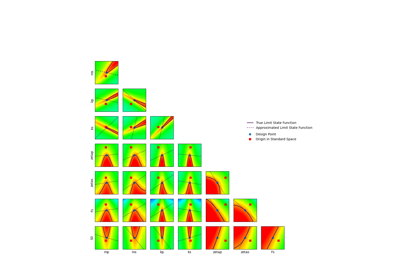
We consider a two degree-of-fredom primary-secondary damped oscillator. This system is composed of a two-stage oscillator characterized by a mass, a stiffness and a damping ratio for each of the two oscillators. This system is submitted to a white-noise excitation. The limit-state function is highly nonlinear, mainly due to the interactions between the two stages of the system, and presents one failure zone.

use case oscillator — Two stage oscillator¶

The limit state function is defined as follows:

$G = F_s - 3 k_s \sqrt{\frac{\pi S_0}{4 \zeta_s \omega_s^3} \left[\frac{\zeta_a \zeta_s}{\zeta_p \zeta_s (4 \zeta_a^2 + \theta^2)+\gamma \zeta_a^2}\frac{(\zeta_p \omega_p^3 + \zeta_s \omega_s^3)\omega_p}{4 \zeta_a \omega_a^4}\right]}$

The natural frequency of the first oscillator is equal to:

$\omega_p = \sqrt{\frac{k_p}{m_p}}$

The natural frequency of the secondary oscillator is equal to:

$\omega_s = \sqrt{\frac{k_s}{m_s}}$

The average natural frequency of the system is equal to:

$\omega_a = \frac{\omega_p+\omega_s}{2}$

The average damping ratio of the system is equal to:

$\zeta_a = \frac{\zeta_p+\zeta_s}{2}$

The mass ratio is equal to:

$\gamma = \frac{m_s}{m_p}$

The tuning parameter of the system is equal to:

$\theta = \frac{\omega_p - \omega_s}{\omega_a}$

Eight uncertainties are considered in the system:

on the masses of the primary and secondary systems ( $m_p$ and $m_s$ ),
on the spring stiffeness of the primary and secondary oscillators ( $k_p$ and $k_s$ ),
on the damping ratios of the primary and secondary systems ( $\zeta_p$ and $\zeta_s$ ),
on the loading capacity of the secondary spring ( $F_s$ ),
on the intensity of the white noise excitation ( $S_0$ ).

We consider the following distribution fResponse of Two-Degree-of-Freedom Systems to White-Noise Base Excitation:

$m_p \sim \text{LogNormalSigmaOverMu}( \mu_{m_p} = 1.5, \delta_{m_p} = 0.1)$
$m_s \sim \text{LogNormalSigmaOverMu}( \mu_{m_s} = 0.01, \delta_{m_s} = 0.1)$
$k_p \sim \text{LogNormalSigmaOverMu}( \mu_{k_p} = 1, \delta_{k_p} = 0.2)$
$k_s \sim \text{LogNormalSigmaOverMu}( \mu_{k_s} = 0.01, \delta_{k_s} = 0.2)$
$\zeta_p \sim \text{LogNormalSigmaOverMu}( \mu_{\zeta_p} = 0.05, \delta_{\zeta_p} = 0.4)$
$\zeta_s \sim \text{LogNormalSigmaOverMu}( \mu_{\zeta_s} = 0.02, \delta_{\zeta_s} = 0.5)$
$F_s \sim \text{LogNormalSigmaOverMu}( \mu_{F_s} = 27.5, \delta_{F_s} = 0.1)$
$S_0 \sim \text{LogNormalSigmaOverMu}( \mu_{S_0} = 100, \delta_{S_0} = 0.1)$

The failure probability is:

$P_f = \Prob{G(m_p,m_s,k_p,k_z,\zeta_p,\zeta_s,F_s,Z_0) \leq 0}.$

The value of $P_f$ is:

$P_f = 3.78 \times 10^{-7}.$

References¶

Der Kiureghian, A. and De Stefano, M. (1991). Efficient Algorithm for Second-Order Reliability Analysis, Journal of engineering mechanics, 117(12), 2904-2923
Dubourg, V., Sudret, B., Deheeger, F. (2013). Metamodel-based importance sampling for structural reliability analysis. Probabilistic Engineering Mechanics, 33, pp. 47–57

API documentation¶

class Oscillator

Data class for the oscillator example.

Attributes:

dimint: dim = 8, dimension of the problem
modelSymbolicFunction: The limit state function
muMpfloat: muMp = 1.5, mean of the mass of the primary system
sigmaOverMuMpfloat: sigmaOverMuMp = 0.1, coefficient of variation of the mass of the primary system
distributionMpLogNormal: Distribution of the mass of the primary system distributionMp = ot.LogNormalMuSigmaOverMu(muMp, sigmaOverMuMp).getDistribution()
muMsfloat: muMs = 0.01, mean of the mass of the primary system
sigmaOverMuMsfloat: sigmaOverMuMs = 0.1, coefficient of variation of the mass of the primary system
distributionMsLogNormal: Distribution of the mass of the secondary system distributionMs = ot.LogNormalMuSigmaOverMu(muMs, sigmaOverMuMs).getDistribution()
muKpfloat: muKp = 1, mean of the spring stiffness of the primary system
sigmaOverMuKpfloat: sigmaOverMuKp = 0.2, coefficient of variation of the spring stiffness of the primary system
distributionKpLogNormal: Distribution of the spring stiffness of the primary system distributionKp = ot.LogNormalMuSigmaOverMu(muKp, sigmaOverMuKp).getDistribution()
muKsfloat: muKs = 0.01, mean of the spring stiffness of the secondary system
sigmaOverMuKsfloat: sigmaOverMuKs = 0.2, coefficient of variation of the spring stiffness of the secondary system
distributionKsLogNormal: Distribution of the spring stiffness of the secondary system distributionKs = ot.LogNormalMuSigmaOverMu(muKs, sigmaOverMuKs).getDistribution()
muZetapfloat: muZetap = 0.05, mean of the damping ratio of the primary system
sigmaOverMuZetapfloat: sigmaOverMuZetap = 0.4, coefficient of variation of the damping ratio of the primary system
distributionZetapLogNormal: Distribution of the damping ratio of the primary system distributionZetap = ot.LogNormalMuSigmaOverMu(muZetap, sigmaOverMuZetap).getDistribution()
muZetasfloat: muZetas = 0.02, mean of the damping ratio of the secondary system
sigmaOverMuZetasfloat: sigmaOverMuZetas = 0.5, coefficient of variation of the damping ratio of the secondary system
distributionZetasLogNormal: Distribution of the damping ratio of the secondary system distributionZetas = ot.LogNormalMuSigmaOverMu(muZetas, sigmaOverMuZetas).getDistribution()
muFsfloat: muFs = 27.5, mean of the loading capacity of the secondary spring
sigmaOverFsfloat: sigmaOverFs = 0.1, coefficient of variation of the loading capacity of the secondary spring
distributionFsLogNormal: Distribution of the loading capacity of the secondary spring distributionFs = ot.LogNormalMuSigmaOverMu(muFs, sigmaOverFs).getDistribution()
muS0float: muS0 = 100, mean of the intensity of the white noise
sigmaOverS0float: sigmaOverS0 = 0.1, coefficient of variation of the intensity of the white noise
distributionS0LogNormal: Distribution of the intensity of the white noise distributionS0 = ot.LogNormalMuSigmaOverMu(muS0, sigmaOverS0).getDistribution()
distributionJointDistribution: The joint distribution of the input parameters

Examples

>>> from openturns.usecases import oscillator
>>> # Load the oscillator
>>> osc = oscillator.Oscillator()

Examples based on this use case¶

Using the FORM - SORM algorithms on a nonlinear function

OpenTURNS

An Open source initiative for the Treatment of Uncertainties, Risks'N Statistics

Table of Contents

Previous topic

Next topic

This Page

A two degree-of-fredom primary/secondary damped oscillator¶

References¶

API documentation¶

Examples based on this use case¶