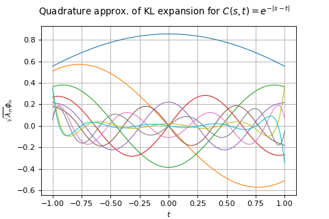
KarhunenLoeveQuadratureAlgorithm¶

(Source code, png)

class KarhunenLoeveQuadratureAlgorithm(*args)¶

Computation of Karhunen-Loeve decomposition using Quadrature approximation.

Available constructors:

KarhunenLoeveQuadratureAlgorithm(domain, bounds, covariance, experiment, basis, basisSize, mustScale, s)

KarhunenLoeveQuadratureAlgorithm(domain, bounds, covariance, marginalDegree, s)

Parameters:

domainDomain: The domain on which the covariance model and the Karhunen-Loeve eigenfunctions (modes) are discretized.
boundsInterval: Numerical bounds of the domain.
covarianceCovarianceModel: The covariance function to decompose.
experimentWeightedExperiment: The points and weights used in the quadrature approximation.
basissequence of Function: The basis in which the eigenfunctions are projected.
marginalDegreeint: The maximum degree to take into account in the tensorized Legendre basis.
mustScalebool: Flag to tell if the bounding box of the weighted experiment and the domain have to be maped or not.
sfloat, $\geq0$: The threshold used to select the most significant eigenmodes, defined in KarhunenLoeveAlgorithm.

Methods

`getBasis`()	Accessor to the functional basis.
`getClassName`()	Accessor to the object's name.
`getCovarianceModel`()	Accessor to the covariance model.
`getDomain`()	Accessor to the domain.
`getExperiment`()	Accessor to the points and weights of the quadrature approximation.
`getMustScale`()	Accessor to scale option.
`getName`()	Accessor to the object's name.
`getNbModes`()	Accessor to number of modes to compute.
`getResult`()	Get the result structure.
`getThreshold`()	Accessor to the threshold used to select the most significant eigenmodes.
`hasName`()	Test if the object is named.
`run`()	Computation of the eigenvalues and eigenfunctions values at the quadrature points.
`setCovarianceModel`(covariance)	Accessor to the covariance model.
`setName`(name)	Accessor to the object's name.
`setNbModes`(nbModes)	Accessor to the maximum number of modes to compute.
`setThreshold`(threshold)	Accessor to the limit ratio on eigenvalues.

Notes

The Karhunen-Loeve quadrature algorithm solves the Fredholm problem associated to the covariance function $C$ : see KarhunenLoeveAlgorithm to get the notations.

The Karhunen-Loeve quadrature approximation consists in replacing the integral by a quadrature approximation: if $(\omega_\ell, \vect{\xi}_\ell)_{1 \leq \ell \leq L}$ is the weighted experiment (see WeightedExperiment) associated to the measure $\mu$ , then for all functions measurable wrt $\mu$ , we have:

$\int_{\Rset^n} f(\vect{x}) \mu(\vect{x})\, d\vect{x} \simeq \sum_{\ell=1}^{\ell=L} \omega_\ell f(\vect{\xi}_\ell)$

If we note $\eta_{\ell}=\omega_{\ell}\dfrac{1_{\cD}(\vect{\xi}_{\ell})}{\mu(\vect{\xi}_{\ell})}$ , we build a more general quadrature approximation $(\eta_\ell, \xi_\ell)_{1 \leq l \leq L}$ such that:

$\int_{\cD} f(\vect{t}) \, d\vect{t} \simeq \sum_{\ell=1}^L \eta_\ell f(\vect{\xi}_\ell)$

where only the points $\vect{\xi}_\ell \in \cD$ are considered.

We introduce the matrices $\mat{\Theta}=(\mat{\Theta}_{ij})_{1 \leq i \leq L, 1 \leq j \leq P} \in \cM_{Ld, Pd}(\Rset)$ such that $\mat{\Theta}_{ij} = \theta_{j}(\vect{\xi}_i)\mat{I}_d$ , $\mat{C}_{\ell, \ell'} = \mat{C}(\vect{\xi}_{\ell},\vect{\xi}_{\ell'})$ and $\mat{W}= \mathrm{diag} (\mat{W}_{ii})_{1 \leq i \leq L} \in \cM_{Ld, Ld}(\Rset)$ such that $\mat{W}_{ii} = \eta_i \mat{I}_d$ .

The normalisation constraint $\|\vect{\varphi}_k\|^2_{L^2(\cD, \Rset^d)}=1$ and the orthogonality of the $\vect{\varphi}_k$ in $L^2(\cD, \Rset^d)$ leads to:

(1)¶ $\Tr{\vect{\Phi}} \,\Tr{\mat{\Theta}} \,\mat{W}\, \mat{\Theta} \,\vect{\Phi}=\mat{I}$

The Galerkin approach leads to the following generalized eigenvalue problem:

(2)¶ $\Tr{\mat{\Theta}} \,\mat{W} \,\mat{C} \,\mat{W} \,\mat{\Theta}\,\vect{\Phi}_k = \lambda_k \Tr{\mat{\Theta}}\, \mat{W}\,\mat{\Theta}\,\vect{\Phi}_k$

where $\Tr{\mat{\Theta}}\, \mat{W} \,\mat{C} \, \mat{W}\, \mat{\Theta}$ and $\Tr{\mat{\Theta}}\, \mat{W}\, \mat{\Theta}\in \cM_{Pd,Pd}(\Rset)$ .

The collocation approach leads to the following generalized eigenvalue problem:

(3)¶ $\mat{C}\, \mat{W} \,\mat{\Theta}\, \vect{\Phi}_k = \lambda_k \mat{\Theta}\,\vect{\Phi}_k$

Equations (2) and (3) are equivalent when $\mat{\Theta}$ is invertible.

OpenTURNS solves the equation (2).

The second constructor is a short-hand to the first one, where basis is the tensorized Legendre basis (see OrthogonalProductPolynomialFactory and LegendreFactory), experiment is a tensorized Gauss-Legendre quadrature (see GaussProductExperiment), basisSize is equal to marginalDegree to the power the dimension of domain and mustScale is set to True.

Examples

Discretize the domain $\cD$ and create a covariance model:

>>> import openturns as ot
>>> bounds = ot.Interval([-1.0]*2, [1.0]*2)
>>> domain = ot.MeshDomain(ot.IntervalMesher([10]*2).build(bounds))
>>> s = 0.01
>>> model = ot.AbsoluteExponential([1.0]*2)

Give the basis used to decompose the eigenfunctions:

here, the 10 first Legendre polynomials family:

>>> basis = ot.OrthogonalProductPolynomialFactory([ot.LegendreFactory()]*2)
>>> functions = [basis.build(i) for i in range(10)]

Create the weighted experiment of the quadrature approximation: here, a Monte Carlo experiment from the measure orthogonal wrt the Legendre polynomials family:

>>> experiment = ot.MonteCarloExperiment(basis.getMeasure(), 1000)

Create the Karhunen-Loeve Quadrature algorithm:

>>> algorithm = ot.KarhunenLoeveQuadratureAlgorithm(domain, bounds, model, experiment, functions, True, s)

Run it!

>>> algorithm.run()
>>> result = algorithm.getResult()

__init__(*args)¶

getBasis()¶

Accessor to the functional basis.

Returns:

basisBasis: The basis in which the eigenfunctions are projected.

getClassName()¶

Accessor to the object’s name.

Returns:

class_namestr: The object class name (object.__class__.__name__).

getCovarianceModel()¶

Accessor to the covariance model.

Returns:

covModelCovarianceModel: The covariance model.

getDomain()¶

Accessor to the domain.

Returns:

domainDomain
The domain $\cD_N$ that discretizes the domin $\cD$ .

getExperiment()¶

Accessor to the points and weights of the quadrature approximation.

Returns:

experimentWeightedExperiment: The points and weights used in the quadrature approximation.

getMustScale()¶

Accessor to scale option.

Returns:

mustScalebool: Flag to tell if the bounding box of the weighted experiment and the domain have to be maped or not.

getName()¶

Accessor to the object’s name.

Returns:

namestr: The name of the object.

getNbModes()¶

Accessor to number of modes to compute.

Returns:

nint: The maximum number of modes to compute. The actual number of modes also depends on the threshold criterion.

getResult()¶

Get the result structure.

Returns:

resKLKarhunenLoeveResult: The structure containing all the results of the Fredholm problem.

Notes

The structure contains all the results of the Fredholm problem.

getThreshold()¶

Accessor to the threshold used to select the most significant eigenmodes.

Returns:

sfloat, positive: The threshold $s$ .

Notes

OpenTURNS truncates the sequence $(\lambda_k, \vect{\varphi}_k)_{k \geq 1}$ at the index $K$ defined in (3).

hasName()¶

Test if the object is named.

Returns:

hasNamebool: True if the name is not empty.

run()¶

Computation of the eigenvalues and eigenfunctions values at the quadrature points.

Notes

Runs the algorithm and creates the result structure KarhunenLoeveResult.

setCovarianceModel(covariance)¶

Accessor to the covariance model.

Parameters:

covModelCovarianceModel: The covariance model.

setName(name)¶

Accessor to the object’s name.

Parameters:

namestr: The name of the object.

setNbModes(nbModes)¶

Accessor to the maximum number of modes to compute.

Parameters:

nint: The maximum number of modes to compute. The actual number of modes also depends on the threshold criterion.

setThreshold(threshold)¶

Accessor to the limit ratio on eigenvalues.

Parameters:

sfloat, $\geq 0$: The threshold $s$ defined in (3).

OpenTURNS

An Open source initiative for the Treatment of Uncertainties, Risks'N Statistics

Previous topic

Next topic

This Page

KarhunenLoeveQuadratureAlgorithm¶