GaussProductExperiment
(Source code, png)
- class GaussProductExperiment(*args)
Gauss product experiment.
- Available constructors:
GaussProductExperiment(marginalSizes)
GaussProductExperiment(distribution)
GaussProductExperiment(distribution, marginalSizes)
- Parameters:
- marginalSizessequence of positive int
Numbers of nodes
for each direction. Then, the total number of nodes generated is
. By default, the value of
is equal to
. The default marginal size is defined in the GaussProductExperiment-DefaultMarginalSize key of the
ResourceMap.- distribution
Distribution
of dimension
with an independent copula.
Methods
generate()Generate points according to the type of the experiment.
Generate points and their associated weight according to the type of the experiment.
Accessor to the object's name.
Accessor to the distribution.
Get the marginal sizes.
getName()Accessor to the object's name.
getSize()Accessor to the size of the generated sample.
hasName()Test if the object is named.
Ask whether the experiment has uniform weights.
isRandom()Accessor to the randomness of quadrature.
setDistribution(distribution)Accessor to the distribution.
setMarginalSizes(marginalSizes)Set the marginal sizes.
setName(name)Accessor to the object's name.
setSize(size)Accessor to the size of the generated sample.
Notes
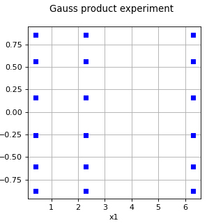
The Gauss product experiment is a tensor product experiment which uses Gauss nodes in each direction. Using the notations of the
TensorProductExperimentdocumentation, the number of marginal experiments is equal toand the dimension of each marginal experiment is
for every index
.
For each marginal, the algorithm computes the family of orthogonal polynomials depending on the marginal distribution using the
StandardDistributionPolynomialFactoryclass. The input distribution must have an independent copula.The
GaussLegendreclass provides a simple algorithm to use Gaussian quadrature with Legendre polynomials.Polynomial exactness
The Gauss tensor product quadrature rule is exact for polynomials up to some degree. More precisely, for any
, let
be the set of mono-variable polynomials of degree lower or equal to
. Consider the tensor product of 1D polynomials:
Therefore the Gauss-Legendre tensorized quadrature is exact for all polynomials of the vector space:
Examples
>>> import openturns as ot
>>> marginal_1 = ot.Exponential()
>>> marginal_2 = ot.Triangular(-1.0, -0.5, 1.0)
>>> distribution = ot.JointDistribution([marginal_1, marginal_2])
>>> marginalSizes = [3, 2]
>>> experiment = ot.GaussProductExperiment(distribution, marginalSizes)
>>> nodes, weights = experiment.generateWithWeights()
>>> print(nodes)
    [ X0        X1        ]
0 : [  0.415775 -0.511215 ]
1 : [  2.29428  -0.511215 ]
2 : [  6.28995  -0.511215 ]
3 : [  0.415775  0.357369 ]
4 : [  2.29428   0.357369 ]
5 : [  6.28995   0.357369 ]
>>> print(weights)
[0.429018,0.168036,0.00626806,0.282075,0.110482,0.00412119]
In the following example [morokoff1995], we integrate a dimension 5 integrand with
marginal probability density functions. We use 7 nodes for each marginal, leading to a total of
nodes for the tensor product Gauss quadrature.
>>> import openturns as ot
>>> def g_function_py(x):
...     value = (1.0 + 1.0 / dimension) ** dimension
...     for i in range(dimension):
...         value *= x[i] ** (1.0 / dimension)
...     return [value]
>>>
>>> dimension = 5
>>> g_function = ot.PythonFunction(dimension, 1, g_function_py)
>>> interval = ot.Interval([0.0] * dimension, [1.0] * dimension)
>>> integral = 1.0
>>> print('Exact integral = ', integral)
Exact integral =  1.0
>>> marginal_levels = [7] * dimension
>>> distribution = ot.JointDistribution([ot.Uniform(0.0, 1.0)] * dimension)
>>> experiment = ot.GaussProductExperiment(distribution, marginal_levels)
>>> nodes, weights = experiment.generateWithWeights()
>>> number_of_nodes = nodes.getSize()
>>> print('Number of nodes = ', number_of_nodes)
Number of nodes =  16807
>>> function_values = g_function(nodes).asPoint()
>>> approximate_integral = function_values.dot(weights)
>>> print('Approximate integral = ', approximate_integral)
Approximate integral =  1.0040...
- __init__(*args)
- generate()
Generate points according to the type of the experiment.
- Returns:
- sample
Sample Points
of the design of experiments. The sampling method is defined by the type of the weighted experiment.
- sample
Examples
>>> import openturns as ot
>>> ot.RandomGenerator.SetSeed(0)
>>> myExperiment = ot.MonteCarloExperiment(ot.Normal(2), 5)
>>> sample = myExperiment.generate()
>>> print(sample)
    [ X0        X1        ]
0 : [  0.608202 -1.26617  ]
1 : [ -0.438266  1.20548  ]
2 : [ -2.18139   0.350042 ]
3 : [ -0.355007  1.43725  ]
4 : [  0.810668  0.793156 ]
- generateWithWeights()
Generate points and their associated weight according to the type of the experiment.
- Returns:
Examples
>>> import openturns as ot
>>> ot.RandomGenerator.SetSeed(0)
>>> myExperiment = ot.MonteCarloExperiment(ot.Normal(2), 5)
>>> sample, weights = myExperiment.generateWithWeights()
>>> print(sample)
    [ X0        X1        ]
0 : [  0.608202 -1.26617  ]
1 : [ -0.438266  1.20548  ]
2 : [ -2.18139   0.350042 ]
3 : [ -0.355007  1.43725  ]
4 : [  0.810668  0.793156 ]
>>> print(weights)
[0.2,0.2,0.2,0.2,0.2]
- getClassName()
Accessor to the object’s name.
- Returns:
- class_namestr
The object class name (object.__class__.__name__).
- getDistribution()
Accessor to the distribution.
- Returns:
- distribution
Distribution Distribution of the input random vector.
- distribution
- getMarginalSizes()
Get the marginal sizes.
- Returns:
- marginalSizes
Indices Numbers of points
for each direction.
- marginalSizes
- getName()
Accessor to the object’s name.
- Returns:
- namestr
The name of the object.
- getSize()
Accessor to the size of the generated sample.
- Returns:
- sizepositive int
Number
of points constituting the design of experiments.
- hasName()
Test if the object is named.
- Returns:
- hasNamebool
True if the name is not empty.
- hasUniformWeights()
Ask whether the experiment has uniform weights.
- Returns:
- hasUniformWeightsbool
Whether the experiment has uniform weights.
- isRandom()
Accessor to the randomness of quadrature.
- Parameters:
- isRandombool
Is true if the design of experiments is random. Otherwise, the design of experiment is assumed to be deterministic.
- setDistribution(distribution)
Accessor to the distribution.
- Parameters:
- distribution
Distribution Distribution of the input random vector.
- distribution
- setMarginalSizes(marginalSizes)
Set the marginal sizes.
- Parameters:
- marginalSizessequence of positive int
Numbers of points
for each direction.
- setName(name)
Accessor to the object’s name.
- Parameters:
- namestr
The name of the object.
- setSize(size)
Accessor to the size of the generated sample.
- Parameters:
- sizepositive int
Number
of points constituting the design of experiments. Only available in dimension 1.
Examples using the class
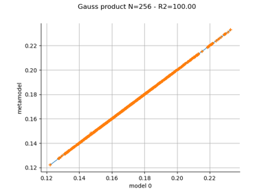
Create a polynomial chaos metamodel by integration on the cantilever beam
 OpenTURNS

