KernelSmoothing¶

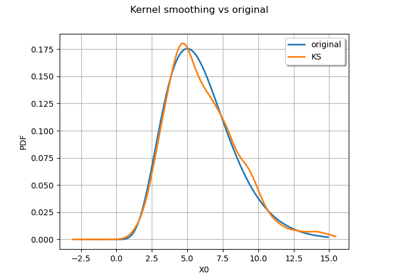
(Source code, png)

class KernelSmoothing(*args)¶

Non parametric continuous distribution estimation by kernel smoothing.

Parameters:

kernelDistribution, optional: Univariate distribution of the kernel that will be used. By default, the standard Normal distribution is used.
binnedbool, optional: Activates bining mechanism only in the univariate or bivariate cases. It allows one to speed up the manipulation of the density function of the resulting distribution. By default, the mechanism is activated.
binNumberint, $binNumber \geq 2$ , optional: Indicates the number of bins used by the bining mechanism. By default, OpenTURNS uses the values stored in ResourceMap.
boundaryCorrectionbool, optional: Activates the boundary correction using the mirroring technique. By default, the correction is not provided.

Methods

`build`(*args)	Fit a kernel smoothing distribution on data.
`buildAsKernelMixture`(sample, bandwidth)	Fit a kernel smoothing distribution on data.
`buildAsMixture`(sample, bandwidth)	Fit a kernel smoothing distribution on data.
`buildAsTruncatedDistribution`(sample, bandwidth)	Estimate the distribution as `TruncatedDistribution`.
`buildEstimator`(*args)	Build the distribution and the parameter distribution.
`computeMixedBandwidth`(sample)	Compute the bandwidth according to a mixed rule.
`computePluginBandwidth`(sample)	Compute the bandwidth according to the plugin rule.
`computeSilvermanBandwidth`(sample)	Compute the bandwidth according to the Silverman rule.
`getBandwidth`()	Accessor to the bandwidth used in the kernel smoothing.
`getBinNumber`()	Accessor to the bin number.
`getBinning`()	Accessor to the binning flag.
`getBootstrapSize`()	Accessor to the bootstrap size.
`getBoundaryCorrection`()	Accessor to the boundary correction flag.
`getClassName`()	Accessor to the object's name.
`getKernel`()	Accessor to kernel used in the kernel smoothing.
`getKnownParameterIndices`()	Accessor to the known parameters indices.
`getKnownParameterValues`()	Accessor to the known parameters values.
`getName`()	Accessor to the object's name.
`getUseLogTransform`()	Accessor to the log-transform flag.
`hasName`()	Test if the object is named.
`setAutomaticLowerBound`(automaticLowerBound)	Accessor to the flag for an automatic selection of lower bound.
`setAutomaticUpperBound`(automaticUpperBound)	Accessor to the flag for an automatic selection of upper bound.
`setBinNumber`(binNumber)	Accessor to the bin number.
`setBinning`(binned)	Accessor to the binning flag.
`setBootstrapSize`(bootstrapSize)	Accessor to the bootstrap size.
`setBoundaryCorrection`(boundaryCorrection)	Accessor to the boundary correction flag.
`setBoundingOption`(boundingOption)	Accessor to the boundary correction option.
`setKnownParameter`(values, positions)	Accessor to the known parameters.
`setLowerBound`(lowerBound)	Accessor to the lower bound for boundary correction.
`setName`(name)	Accessor to the object's name.
`setUpperBound`(upperBound)	Accessor to the upper bound for boundary correction.
`setUseLogTransform`(useLog)	Accessor to the log-transform flag.

Notes

The binning mechanism is available in dimension 1 and 2 only. See the notes of the setBinning() method for details.

The boundary correction is available in dimension 1 only, and it is done using the mirroring technique (also named as the reflection correction). See the notes of the setBoundingOption() method for details.

It is possible to apply a log-transformation on the data in dimension 1 only, and build the kernel smoothing distribution on the transformed data. See the notes of the setUseLogTransform() method for details.

When applied to multivariate samples, the kernel is the kernel product of the univariate distribution specified in the constructor.

Examples

Fit a distribution on data thanks to the kernel smoothing technique:

>>> import openturns as ot
>>> ot.RandomGenerator.SetSeed(0)
>>> sample = ot.Gamma(6.0, 1.0).getSample(100)
>>> ks = ot.KernelSmoothing()
>>> fittedDist = ks.build(sample)
>>> print(fittedDist.getClassName())
Distribution

The build() method produces a generic Distribution object. Other build methods (detailed below) produce more specific objects.

Get the bandwidth:

>>> bandwidth = ks.getBandwidth()
>>> print(bandwidth)
[0.862207]

The bandwidth was evaluated by the build() method. It could also have been provided by the user.

>>> bandwidth = [0.9]
>>> fittedDist = ks.build(sample, bandwidth)

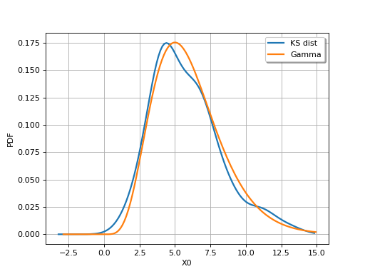
Compare the PDFs:

>>> graph = fittedDist.drawPDF()
>>> graph.add( ot.Gamma(6.0, 1.0).drawPDF())
>>> graph.setLegends(['KS dist', 'Gamma'])

The default values of the parameters of the constructor usually provide good results. Nevertheless, the parameters can be manually set.

>>> kernel = ot.Uniform()
>>> ks = ot.KernelSmoothing(kernel)
>>> binned = True # by default True
>>> binNumber = 64
>>> ks = ot.KernelSmoothing(kernel, binned, binNumber)
>>> boundaryCorrection = True # by default False
>>> ks = ot.KernelSmoothing(kernel, binned, binNumber, boundaryCorrection)

Variants of the build() method can be used when the distribution to build is expected to be of a certain type. In those cases however, the bandwidth must be user-specified. To use buildAsTruncatedDistribution(), boundary correction must be activated. To use the LogTransform treatment, activate it with setUseLogTransform().

>>> distribution = ks.buildAsKernelMixture(sample, bandwidth)
>>> print(distribution.getClassName())
KernelMixture
>>> distribution = ks.buildAsMixture(sample, bandwidth)
>>> print(distribution.getClassName())
Mixture
>>> distribution = ks.buildAsTruncatedDistribution(sample, bandwidth)
>>> print(distribution.getClassName())
TruncatedDistribution
>>> ks.setUseLogTransform(True)
>>> distribution = ks.build(sample)
>>> print(distribution.getClassName())
Distribution

__init__(*args)¶

build(*args)¶

Fit a kernel smoothing distribution on data.

Parameters:

sample2-d sequence of float: Data on which the distribution is fitted. Any dimension.
bandwidthPoint, optional: Contains the bandwidth in each direction. If not specified, the bandwidth is calculated using the mixed rule from data.

Returns:

fittedDistDistribution: The fitted distribution.

Notes

According to the dimension of the data and the specified treatments, the resulting distribution differs.

If the sample is constant, a Dirac distribution is built.
In dimension 1:
- if no treatment is activated, a KernelMixture is built by using buildAsKernelMixture(),
- if a boundary treatment is activated, a TruncatedDistribution is built by using buildAsTruncatedDistribution(),
- if a log-transformation is activated, a CompositeDistribution is built by using build().
In dimension > 2:
- no treatment (boundary correction or log-transformation) is available. A KernelMixture is built by using buildAsKernelMixture().
In dimension 1 or 2, if a binning treatment is activated:
- If the sample size is greater than the bin number, then a Mixture is built by using buildAsMixture(),
- Otherwise a KernelMixture is built by using buildAsKernelMixture().

The bandwidth selection depends on the dimension:

If dimension 1, then computeMixedBandwidth() is used,

Otherwise, then the only multivariate rule computeSilvermanBandwidth() is used.

Examples

See the effect of the boundary correction:

>>> import openturns as ot
>>> sample = ot.Exponential(1.0).getSample(1000)
>>> smoother = ot.KernelSmoothing()
>>> fittedDistNoCorr = smoother.build(sample)
>>> smoother.setBoundaryCorrection(True)
>>> fittedDistWithCorr = smoother.build(sample)

Compare the PDFs:

>>> graph = ot.Exponential(1.0).drawPDF()
>>> graph.add(fittedDistNoCorr.drawPDF())
>>> graph.add(fittedDistWithCorr.drawPDF())
>>> graph.setLegends(['Exp dist', 'No boundary corr', 'Boundary corr'])

buildAsKernelMixture(sample, bandwidth)¶

Fit a kernel smoothing distribution on data.

Parameters:

sample2-d sequence of float: Data on which the distribution is fitted. Any dimension.
bandwidthPoint: Contains the bandwidth in each direction.

Returns:

fittedDistKernelMixture: The fitted distribution.

Notes

It builds a KernelMixture using the given data and bandwidth regardless of the binning or boundary treatment flags.

Examples

>>> import openturns as ot
>>> sample = ot.Exponential(1.0).getSample(1000)
>>> smoother = ot.KernelSmoothing()
>>> kernelMixture = smoother.buildAsKernelMixture(sample, [1.0])

buildAsMixture(sample, bandwidth)¶

Fit a kernel smoothing distribution on data.

Parameters:

sample2-d sequence of float: Data on which the distribution is fitted. Any dimension.
bandwidthPoint: Contains the bandwidth in each direction.

Returns:

fittedDistMixture: The fitted distribution.

Notes

It builds a Mixture using the given bandwidth and a binning of the given data regardless of the bin number, the data size, the binning flag or boundary treatment flags. This method is available only for 1D or 2D samples.

Examples

>>> import openturns as ot
>>> sample = ot.Exponential(1.0).getSample(1000)
>>> smoother = ot.KernelSmoothing(ot.Normal(), True, 100, False)
>>> mixture = smoother.buildAsMixture(sample, [1.0])

buildAsTruncatedDistribution(sample, bandwidth)¶

Estimate the distribution as TruncatedDistribution.

Parameters:

sample2-d sequence of float: Data on which the distribution is fitted. Any dimension.
bandwidthPoint: Contains the bandwidth in each direction.

Returns:

fittedDistTruncatedDistribution: The estimated distribution as a TruncatedDistribution.

Examples

>>> import openturns as ot
>>> sample = ot.Exponential(1.0).getSample(1000)
>>> smoother = ot.KernelSmoothing(ot.Normal(), False, 0, True)
>>> truncated = smoother.buildAsTruncatedDistribution(sample, [1.0])

buildEstimator(*args)¶

Build the distribution and the parameter distribution.

Parameters:

sample2-d sequence of float: Data.
parametersDistributionParameters: Optional, the parametrization.

Returns:

resDistDistributionFactoryResult: The results.

Notes

According to the way the native parameters of the distribution are estimated, the parameters distribution differs:

Moments method: the asymptotic parameters distribution is normal and estimated by Bootstrap on the initial data;

Maximum likelihood method with a regular model: the asymptotic parameters distribution is normal and its covariance matrix is the inverse Fisher information matrix;

Other methods: the asymptotic parameters distribution is estimated by Bootstrap on the initial data and kernel fitting (see KernelSmoothing).

If another set of parameters is specified, the native parameters distribution is first estimated and the new distribution is determined from it:

if the native parameters distribution is normal and the transformation regular at the estimated parameters values: the asymptotic parameters distribution is normal and its covariance matrix determined from the inverse Fisher information matrix of the native parameters and the transformation;

in the other cases, the asymptotic parameters distribution is estimated by Bootstrap on the initial data and kernel fitting.

computeMixedBandwidth(sample)¶

Compute the bandwidth according to a mixed rule.

Returns:

bandwidthPoint: Bandwidth which components are evaluated according to a mixed rule.

Notes

This method uses the mixed rule introduced in Kernel smoothing. Its goal is to provide an accurate estimator of the bandwidth when the sample size is large.

Let $\sampleSize$ be the sample size. The estimator depends on the threshold sample size $n_t$ defined in the KernelSmoothing-SmallSize key of the ResourceMap:

if $\sampleSize \leq n_t$ , i.e. for a small sample, we use the plugin solve-the-equation method,
otherwise, the mixed rule is used.

computePluginBandwidth(sample)¶

Compute the bandwidth according to the plugin rule.

Returns:

bandwidthPoint: Bandwidth computed according to the plug-in rule.

Notes

Each component of the bandwidth which components is evaluated according to the plug-in rule. This plug-in rule is based on the solve-the-equation method from [sheather1991]. This method can take a lot of time for large samples, as the cost is quadratic with the sample size.

Several keys of the ResourceMap are used by the [sheather1991] method.

The key KernelSmoothing-AbsolutePrecision is used in the Sheather-Jones algorithm to estimate the bandwidth. It defines the absolute tolerance used by the solver to solve the nonlinear equation.
The KernelSmoothing-MaximumIteration key defines the maximum number of iterations used by the solver.
The KernelSmoothing-RelativePrecision key defines the relative tolerance.
The KernelSmoothing-AbsolutePrecision key defines the absolute tolerance.
The KernelSmoothing-ResidualPrecision key defines the absolute tolerance on the residual.
The KernelSmoothing-CutOffPlugin key is the cut-off value introduced in Kernel smoothing.

More precisely, the KernelSmoothing-CutOffPlugin key of the ResourceMap controls the accuracy of the approximation used to estimate the rugosity of the second derivative of the distribution. The default value ensures that terms in the sum which weight are lower than $4 \times 10^{-6}$ are ignored, which can reduce the calculation in some situations. The properties of the standard gaussian density are so that, in order to make the computation exact, the value of the KernelSmoothing-CutOffPlugin must be set to 39, but this may increase the computation time.

computeSilvermanBandwidth(sample)¶

Compute the bandwidth according to the Silverman rule.

Returns:

bandwidthPoint: Bandwidth computed according to the Silverman rule.

Notes

Each component of the bandwidth which components is evaluated according to the Silverman rule assuming a normal distribution. The bandwidth uses a robust estimate of the sample standard deviation, based on the interquartile range introduced in Kernel smoothing (rather than the sample standard deviation). This method can manage a multivariate sample and produces a multivariate bandwidth.

getBandwidth()¶

Accessor to the bandwidth used in the kernel smoothing.

Returns:

bandwidthPoint: Bandwidth.

getBinNumber()¶

Accessor to the bin number.

Returns:

binNumberint: The bin number.

getBinning()¶

Accessor to the binning flag.

Returns:

binningbool: Flag to tell if the binning treatment is activated.

Notes

This treatment is available in dimension 1 and 2 only.

getBootstrapSize()¶

Accessor to the bootstrap size.

Returns:

sizeint: Size of the bootstrap.

getBoundaryCorrection()¶

Accessor to the boundary correction flag.

Returns:

boundaryCorrectionbool: Flag to tell if the boundary correction is activated.

Notes

This treatment is available in dimension 1 only.

getClassName()¶

Accessor to the object’s name.

Returns:

class_namestr: The object class name (object.__class__.__name__).

getKernel()¶

Accessor to kernel used in the kernel smoothing.

Returns:

kernelDistribution: Univariate distribution used to build the kernel.

getKnownParameterIndices()¶

Accessor to the known parameters indices.

Returns:

indicesIndices: Indices of the known parameters.

getKnownParameterValues()¶

Accessor to the known parameters values.

Returns:

valuesPoint: Values of known parameters.

getName()¶

Accessor to the object’s name.

Returns:

namestr: The name of the object.

getUseLogTransform()¶

Accessor to the log-transform flag.

Returns:

useLogTransformbool: Flag to tell if the kernel smoothing distribution is built on the log-transformed data.

Notes

This treatment is available in dimension 1 only.

hasName()¶

Test if the object is named.

Returns:

hasNamebool: True if the name is not empty.

setAutomaticLowerBound(automaticLowerBound)¶

Accessor to the flag for an automatic selection of lower bound.

Parameters:

automaticLowerBoundbool: Flag to tell if the lower bound is automatically calculated from the sample.

Notes

This treatment is available in dimension 1 only. The automatic lower bound is the minimum of the given sample. In the other case, the user has to specify the lower bound.

setAutomaticUpperBound(automaticUpperBound)¶

Accessor to the flag for an automatic selection of upper bound.

Parameters:

automaticUpperBoundbool: Flag to tell if the upper bound is automatically calculated from the sample.

Notes

This treatment is available in dimension 1 only. The automatic upper bound is the maximum of the given sample. In the other case, the user has to specify the upper bound.

setBinNumber(binNumber)¶

Accessor to the bin number.

Parameters:

binNumberint: The bin number.

setBinning(binned)¶

Accessor to the binning flag.

Parameters:

binningbool: Flag to tell if the binning treatment is activated.

Notes

This treatment is available in dimension 1 and 2 only. It creates a regular grid of binNumber intervals in each dimension, then the unit weight of each point is linearly affected to the vertices of the bin containing the point (see [wand1994] appendix D, page 182). The KernelSmoothing-BinNumber key of the class ResourceMap defines the default value of the number of bins used in the _binning_ algorithm to improve the evaluation speed.

setBootstrapSize(bootstrapSize)¶

Accessor to the bootstrap size.

Parameters:

sizeint: The size of the bootstrap.

setBoundaryCorrection(boundaryCorrection)¶

Accessor to the boundary correction flag.

Parameters:

boundaryCorrectionbool: Activates the boundary correction using the mirroring technique.

Notes

This treatment is available in dimension 1 only. See [jones1993] to get more details. The reflection or mirroring method is used: the boundaries are automatically detected from the sample (with the Sample.getMin() and Sample.getMax() functions) and the kernel smoothed distribution is corrected in the boundary areas to remain within the boundaries, according to the mirroring technique:

the Scott bandwidth is evaluated from the sample: h
two sub-samples are extracted from the initial sample, containing all the points within the range $[min, min + h[$ and $]max-h, max]$ ,
both sub-samples are transformed into their symmetric samples with respect their respective boundary: its results two samples within the range $]min-h, min]$ and $[max, max+h[$ ,
a kernel smoothed PDF is built from the new sample composed with the initial one and the two new ones, with the previous bandwidth h,
this last kernel smoothed PDF is truncated within the initial range $[min, max]$ (conditional PDF).

setBoundingOption(boundingOption)¶

Accessor to the boundary correction option.

Parameters:

boundingOptionint: Select the boundary correction option, see notes.

Notes

The possible values for the bounding option are:

KernelSmoothing.NONE or 0: no boundary correction

KernelSmoothing.LOWER or 1: apply the boundary correction to the lower bound

KernelSmoothing.UPPER or 2: apply the boundary correction to the upper bound

KernelSmoothing.BOTH or 3: apply the boundary correction to both bounds

This treatment is available in dimension 1 only. Each bound can be defined by the user or computed automatically from the sample, see setLowerBound(), setUpperBound(), setAutomaticLowerBound(), setAutomaticUpperBound().

setKnownParameter(values, positions)¶

Accessor to the known parameters.

Parameters:

valuessequence of float: Values of known parameters.
positionssequence of int: Indices of known parameters.

Examples

When a subset of the parameter vector is known, the other parameters only have to be estimated from data.

In the following example, we consider a sample and want to fit a Beta distribution. We assume that the $a$ and $b$ parameters are known beforehand. In this case, we set the third parameter (at index 2) to -1 and the fourth parameter (at index 3) to 1.

>>> import openturns as ot
>>> ot.RandomGenerator.SetSeed(0)
>>> distribution = ot.Beta(2.3, 2.2, -1.0, 1.0)
>>> sample = distribution.getSample(10)
>>> factory = ot.BetaFactory()
>>> # set (a,b) out of (r, t, a, b)
>>> factory.setKnownParameter([-1.0, 1.0], [2, 3])
>>> inf_distribution = factory.build(sample)

setLowerBound(lowerBound)¶

Accessor to the lower bound for boundary correction.

Parameters:

lowerBoundfloat: A user-defined lower bound to take into account for boundary correction.

Notes

This treatment is available in dimension 1 only. This method automatically sets the automaticLowerBound flag to False. The given value will be taken into account only if boundingOption is set to either 1 or 3. If the algorithm is applied to a sample with a minimum value less than the user-defined lower bound and the automaticLowerBound is set to False, then an exception it raised.

setName(name)¶

Accessor to the object’s name.

Parameters:

namestr: The name of the object.

setUpperBound(upperBound)¶

Accessor to the upper bound for boundary correction.

Parameters:

upperBoundfloat: A user-defined upper bound to take into account for boundary correction.

Notes

This treatment is available in dimension 1 only. This method automatically sets the automaticLowerBound flag to False. The given value will be taken into account only if boundingOption is set to either 1 or 3. If the algorithm is applied to a sample with a minimum value less than the user-defined lower bound and the automaticLowerBound is set to False, then an exception it raised.

setUseLogTransform(useLog)¶

Accessor to the log-transform flag.

Parameters:

useLogTransformbool: Flag to tell if the kernel smoothing distribution is built on the log-transformed data.

Notes

This treatment is available in dimension 1 only. See [charpentier2015] to get more details.

We denote by $(X_i)_{1 \leq i \leq \sampleSize}$ some independent random variates, identically distributed according to $X$ .

Refer to Kernel smoothing for the details. The shift scale is fixed in the KernelSmoothing-DefaultShiftScale key of the class ResourceMap.

Once a kernel smoothed distribution has been fitted on the transformed data, the fitted distribution of $X$ is built as a CompositeDistribution from $T^{-1}$ and the kernel smoothed distribution.