Point¶

class Point(*args)¶

Real vector.

Parameters:

dimensionint, $n > 0$ , optional: The number of components.
valuefloat, optional: The components value. Default creates a null vector.

Methods

`add`(*args)	Append a component (in-place).
`at`(*args)	Access to an element of the collection.
`clear`()	Reset the collection to zero dimension.
`dot`(rhs)	Compute the scalar product.
`find`(val)	Find the index of a given value.
`getClassName`()	Accessor to the object's name.
`getDimension`()	Accessor to the vector's dimension.
`getName`()	Accessor to the object's name.
`getSize`()	Accessor to the vector's dimension (or size).
`hasName`()	Test if the object is named.
`isDecreasing`()	Check if the components are in decreasing order.
`isEmpty`()	Tell if the collection is empty.
`isIncreasing`()	Check if the components are in increasing order.
`isMonotonic`()	Check if the components are in nonincreasing or nondecreasing order.
`isNonDecreasing`()	Check if the components are in nondecreasing order.
`isNonIncreasing`()	Check if the components are in nonincreasing order.
`norm`()	Compute the Euclidean ( $L^2$ ) norm.
`norm1`()	Compute the $L^1$ norm.
`normInf`()	Compute the $L^{\inf}$ norm.
`normSquare`()	Compute the squared Euclidean norm.
`normalize`()	Compute the normalized vector with respect to its Euclidean norm.
`normalizeSquare`()	Compute the normalized vector with respect to its squared Euclidean norm.
`resize`(newSize)	Change the size of the collection.
`select`(marginalIndices)	Selection from indices.
`setName`(name)	Accessor to the object's name.

Examples

Create a Point

>>> import openturns as ot
>>> x = ot.Point(3, 1.0)
>>> x
class=Point name=Unnamed dimension=3 values=[1,1,1]

Get or set terms

>>> print(x[0])
1.0
>>> x[0] = 0.0
>>> print(x[0])
0.0
>>> print(x[:2])
[0,1]

Create a Point from a flat (1d) array, list or tuple

>>> import numpy as np
>>> y = ot.Point((0.0, 1.0, 2.0))
>>> y = ot.Point(range(3))
>>> y = ot.Point(np.arange(3))

and back

>>> z = np.array(y)

Addition, subtraction (with compatible dimensions)

>>> print(x + y)
[0,2,3]
>>> print(x - y)
[0,0,-1]

Multiplication, division with a scalar

>>> print(x * 3.0)
[0,3,3]
>>> print(x / 3.0)
[0,0.333333,0.333333]

__init__(*args)¶

add(*args)¶

Append a component (in-place).

Parameters:

valuetype depends on the type of the collection.: The component to append.

Examples

>>> import openturns as ot
>>> x = ot.Point(2)
>>> x.add(1.)
>>> print(x)
[0,0,1]

at(*args)¶

Access to an element of the collection.

Parameters:

indexpositive int: Position of the element to access.

Returns:

elementtype depends on the type of the collection: Element of the collection at the position index.

clear()¶

Reset the collection to zero dimension.

Examples

>>> import openturns as ot
>>> x = ot.Point(2)
>>> x.clear()
>>> x
class=Point name=Unnamed dimension=0 values=[]

dot(rhs)¶

Compute the scalar product.

Parameters:

pointsequence of float: Scalar product second argument

Returns:

dotfloat: Scalar product

Examples

>>> import openturns as ot
>>> x = ot.Point([1.0, 2.0, 3.0])
>>> prod = x.dot([4, 5, 6])

find(val)¶

Find the index of a given value.

Parameters:

valcollection value type: The value to find

Returns:

indexint: The index of the first occurrence of the value, or the size of the container if not found. When several values match, only the first index is returned.

getClassName()¶

Accessor to the object’s name.

Returns:

class_namestr: The object class name (object.__class__.__name__).

getDimension()¶

Accessor to the vector’s dimension.

Returns:

nint: The number of components in the vector.

getName()¶

Accessor to the object’s name.

Returns:

namestr: The name of the object.

getSize()¶

Accessor to the vector’s dimension (or size).

Returns:

nint: The number of components in the vector.

hasName()¶

Test if the object is named.

Returns:

hasNamebool: True if the name is not empty.

isDecreasing()¶

Check if the components are in decreasing order.

Examples

>>> import openturns as ot
>>> x = ot.Point([3.0, 2.0, 1.0])
>>> x.isDecreasing()
True
>>> x = ot.Point([3.0, 3.0, 1.0])
>>> x.isDecreasing()
False
>>> x = ot.Point([1.0, 3.0, 2.0])
>>> x.isIncreasing()
False

isEmpty()¶

Tell if the collection is empty.

Returns:

isEmptybool: True if there is no element in the collection.

Examples

>>> import openturns as ot
>>> x = ot.Point(2)
>>> x.isEmpty()
False
>>> x.clear()
>>> x.isEmpty()
True

isIncreasing()¶

Check if the components are in increasing order.

Examples

>>> import openturns as ot
>>> x = ot.Point([1.0, 2.0, 3.0])
>>> x.isIncreasing()
True
>>> x = ot.Point([1.0, 1.0, 3.0])
>>> x.isIncreasing()
False
>>> x = ot.Point([1.0, 3.0, 2.0])
>>> x.isIncreasing()
False

isMonotonic()¶

Check if the components are in nonincreasing or nondecreasing order.

Examples

>>> import openturns as ot
>>> x = ot.Point([1.0, 2.0, 3.0])
>>> x.isMonotonic()
True
>>> x = ot.Point([2.0, 2.0, 1.0])
>>> x.isMonotonic()
True
>>> x = ot.Point([1.0, 3.0, 2.0])
>>> x.isMonotonic()
False

isNonDecreasing()¶

Check if the components are in nondecreasing order.

Examples

>>> import openturns as ot
>>> x = ot.Point([1.0, 2.0, 3.0])
>>> x.isNonDecreasing()
True
>>> x = ot.Point([1.0, 1.0, 3.0])
>>> x.isNonDecreasing()
True
>>> x = ot.Point([1.0, 3.0, 2.0])
>>> x.isNonDecreasing()
False

isNonIncreasing()¶

Check if the components are in nonincreasing order.

Examples

>>> import openturns as ot
>>> x = ot.Point([3.0, 2.0, 1.0])
>>> x.isNonIncreasing()
True
>>> x = ot.Point([3.0, 3.0, 1.0])
>>> x.isNonIncreasing()
True
>>> x = ot.Point([1.0, 3.0, 2.0])
>>> x.isNonIncreasing()
False

norm()¶

Compute the Euclidean ( $L^2$ ) norm.

The Euclidean ( $L^2$ ) norm of a vector is defined as:

$\norm{\vect{x}} = \norm{\vect{x}}_2 = \sqrt{\sum_{i=1}^n x_i^2}$

Returns:

normfloat: The vector’s Euclidean norm.

Examples

>>> import openturns as ot
>>> x = ot.Point([1.0, 2.0, 3.0])
>>> x.norm()
3.741657...

norm1()¶

Compute the $L^1$ norm.

The $L^1$ norm of a vector is defined as:

$\norm{\vect{x}}_1 = \sum_{i=1}^n |x_i|$

Returns:

normfloat: The vector’s $L^1$ norm.

Examples

>>> import openturns as ot
>>> x = ot.Point([1.0, 2.0, 3.0])
>>> x.norm1()
6.0

normInf()¶

Compute the $L^{\inf}$ norm.

The $L^{\inf}$ norm of a vector is defined as:

$\norm{\vect{x}}_{\inf} = \max_{i=1}^n |x_i|$

Returns:

normfloat: The vector’s $L^{\inf}$ norm.

Examples

>>> import openturns as ot
>>> x = ot.Point([1.0, 2.0, 3.0])
>>> x.normInf()
3.0

normSquare()¶

Compute the squared Euclidean norm.

Returns:

normfloat: The vector’s squared Euclidean norm.

Examples using the class¶

Randomize the lines of a Sample

Estimate a confidence interval of a quantile

A quick start guide to the Point and Sample classes

Estimate correlation coefficients

Compare unconditional and conditional histograms

Compute squared SRC indices confidence intervals

Estimate a GEV on the Venice sea-levels data

Bandwidth sensitivity in kernel smoothing

Estimate a GPD on the Dow Jones Index data

Fitting a distribution with customized maximum likelihood

Fit a non parametric distribution

Estimate a GEV on the Port Pirie sea-levels data

Estimate a GPD on the daily rainfall data

Estimate a GEV on race times data

Estimate a GEV on the Fremantle sea-levels data

Kolmogorov-Smirnov : understand the statistics

Estimate a scalar ARMA process

Create and draw multivariate distributions

Export a field to VTK

Create a custom covariance model

Draw a field

Trend computation

Export a metamodel

Distribution of estimators in linear regression

Over-fitting and model selection

Create a full or sparse polynomial chaos expansion

Create a polynomial chaos metamodel by integration on the cantilever beam

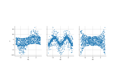
Advanced polynomial chaos construction

Create a polynomial chaos for the Ishigami function: a quick start guide to polynomial chaos

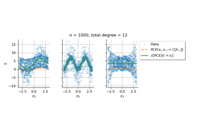
Create a sparse chaos by integration

Conditional expectation of a polynomial chaos expansion

Polynomial chaos expansion cross-validation

Kriging: propagate uncertainties

Kriging : draw the likelihood

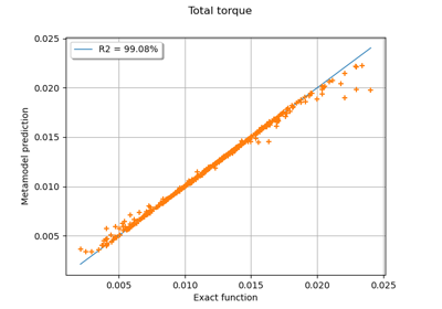
Example of multi output Kriging on the fire satellite model

Kriging: metamodel of the Branin-Hoo function

Sequentially adding new points to a Kriging

Kriging: configure the optimization solver

Kriging: choose a polynomial trend

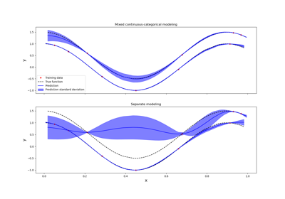
Kriging: metamodel with continuous and categorical variables

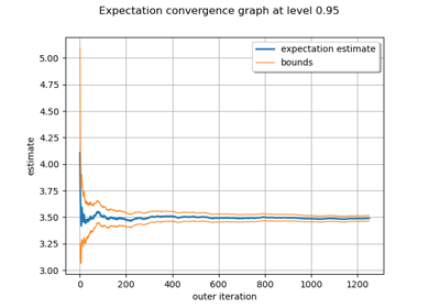
Viscous free fall: metamodel of a field function

Metamodel of a field function

Evaluate the mean of a random vector by simulations

Analyse the central tendency of a cantilever beam

Use the post-analytical importance sampling algorithm

Estimate a flooding probability

Use the Importance Sampling algorithm

Estimate a buckling probability

Exploitation of simulation algorithm results

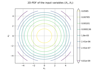
Use the FORM algorithm in case of several design points

Subset Sampling

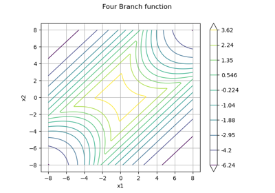
Non parametric Adaptive Importance Sampling (NAIS)

Test the design point with the Strong Maximum Test

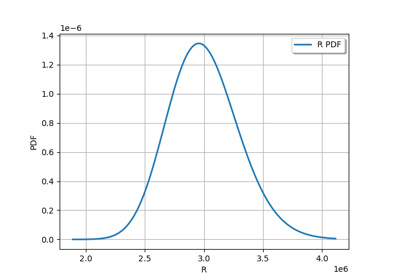
Time variant system reliability problem

Axial stressed beam : comparing different methods to estimate a probability

Cross Entropy Importance Sampling

An illustrated example of a FORM probability estimate

Using the FORM - SORM algorithms on a nonlinear function

Estimate Sobol indices on a field to point function

Sobol’ sensitivity indices using rank-based algorithm

Sobol' sensitivity indices using rank-based algorithm

Estimate Sobol’ indices for the beam by simulation algorithm

Estimate Sobol' indices for the beam by simulation algorithm

FAST sensitivity indices

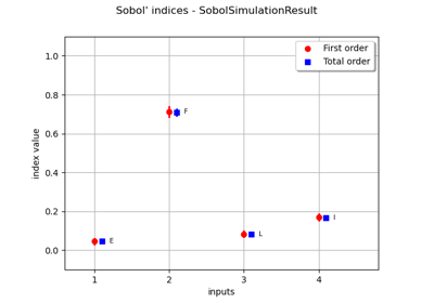
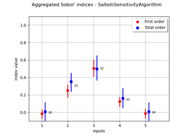
Estimate Sobol’ indices for a function with multivariate output

Estimate Sobol' indices for a function with multivariate output

Use the ANCOVA indices

The HSIC sensitivity indices: the Ishigami model

Example of sensitivity analyses on the wing weight model

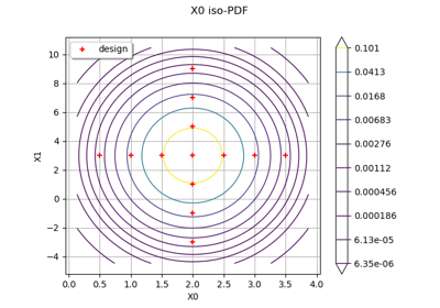
Compute the L2 error between two functions

Create mixed deterministic and probabilistic designs of experiments

Plot the Smolyak quadrature

Use the Smolyak quadrature

Create a composed function

Create an aggregated function

Create a linear combination of functions

Defining Python and symbolic functions: a quick start introduction to functions

Function manipulation

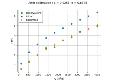
Calibrate a parametric model: a quick-start guide to calibration

Calibration without observed inputs

Calibration of the logistic model

Calibration of the deflection of a tube

Calibration of the flooding model

Calibration of the Chaboche mechanical model

Sampling from an unnormalized probability density

Customize your Metropolis-Hastings algorithm

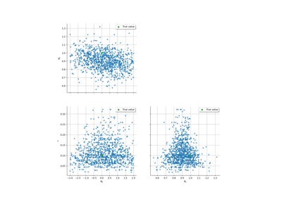
Linear Regression with interval-censored observations

Bayesian calibration of hierarchical fission gas release models

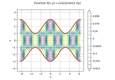
Integrate a function with Gauss-Kronrod algorithm

Estimate a multivariate integral with IteratedQuadrature

Compute leave-one-out error of a polynomial chaos expansion

Compute confidence intervals of a regression model from data

Compute confidence intervals of a univariate noisy function

Mix/max search and sensitivity from design

Quick start guide to optimization

Optimization of the Rastrigin test function

EfficientGlobalOptimization examples

Estimate moments iteratively

Estimate extrema iteratively

Estimate threshold exceedance iteratively

Plot the log-likelihood contours of a distribution

OpenTURNS

An Open source initiative for the Treatment of Uncertainties, Risks'N Statistics

Table of Contents

Previous topic

Next topic

This Page

Point¶

Examples using the class¶