Note

Go to the end to download the full example code.

Estimate a GEV on the Port Pirie sea-levels data¶

In this example, we illustrate various techniques of extreme value modeling applied to the annual maximum sea-levels recorded in Port Pirie, north of Adelaide, south Australia, over the period 1923-1987. Readers should refer to [coles2001] to get more details.

We illustrate techniques to:

estimate a stationary and a non stationary GEV,
estimate a return level,

using:

the log-likelihood function,
the profile log-likelihood function.

First, we load the Port pirie dataset of the annual maximum sea-levels. We start by looking at them through time.

import openturns as ot
import openturns.viewer as otv
from openturns.usecases import coles

data = coles.Coles().portpirie
print(data[:5])
graph = ot.Graph(
    "Annual maximum sea-levels at Port Pirie", "year", "level (m)", True, ""
)
cloud = ot.Cloud(data[:, :2])
cloud.setColor("red")
graph.add(cloud)
graph.setIntegerXTick(True)
view = otv.View(graph)

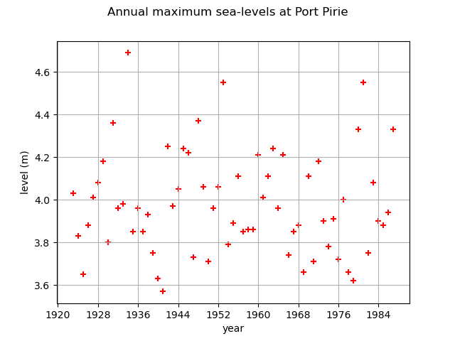
    [ Year     SeaLevel ]
: [ 1923        4.03  ]
: [ 1924        3.83  ]
: [ 1925        3.65  ]
: [ 1926        3.88  ]
: [ 1927        4.01  ]

We select the sea levels column

sample = data[:, 1]

Stationary GEV modeling via the log-likelihood function

We first assume that the dependence through time is negligible, so we first model the data as independent observations over the observation period. We estimate the parameters of the GEV distribution by maximizing the log-likelihood of the data.

factory = ot.GeneralizedExtremeValueFactory()
result_LL = factory.buildMethodOfLikelihoodMaximizationEstimator(sample)

We get the fitted GEV and its parameters of $(\hat{\mu}, \hat{\sigma}, \hat{\xi})$ .

fitted_GEV = result_LL.getDistribution()
desc = fitted_GEV.getParameterDescription()
param = fitted_GEV.getParameter()
print(", ".join([f"{p}: {value:.3f}" for p, value in zip(desc, param)]))
print("log-likelihood = ", result_LL.getLogLikelihood())

mu: 3.875, sigma: 0.198, xi: -0.050
log-likelihood =  4.339057644664945

We get the asymptotic distribution of the estimator $(\hat{\mu}, \hat{\sigma}, \hat{\xi})$ . In that case, the asymptotic distribution is normal.

parameterEstimate = result_LL.getParameterDistribution()
print("Asymptotic distribution of the estimator : ")
print(parameterEstimate)

Asymptotic distribution of the estimator :
Normal(mu = [3.87477,0.198054,-0.0502339], sigma = [0.0269474,0.0236136,0.132905], R = [[  1         0.232937 -0.276996 ]
 [  0.232937  1        -0.466438 ]
 [ -0.276996 -0.466438  1        ]])

We get the covariance matrix and the standard deviation of $(\hat{\mu}, \hat{\sigma}, \hat{\xi})$ .

print("Cov matrix = \n", parameterEstimate.getCovariance())
print("Standard dev = ", parameterEstimate.getStandardDeviation())

Cov matrix =
 [[  0.000726164  0.000148224 -0.000992048 ]
 [  0.000148224  0.000557602 -0.00146386  ]
 [ -0.000992048 -0.00146386   0.0176639   ]]
Standard dev =  [0.0269474,0.0236136,0.132905]

We get the marginal confidence intervals of order 0.95.

order = 0.95
for i in range(3):
    ci = parameterEstimate.getMarginal(i).computeBilateralConfidenceInterval(order)
    print(desc[i] + ":", ci)

mu: [3.82195, 3.92759]
sigma: [0.151772, 0.244336]
xi: [-0.310724, 0.210256]

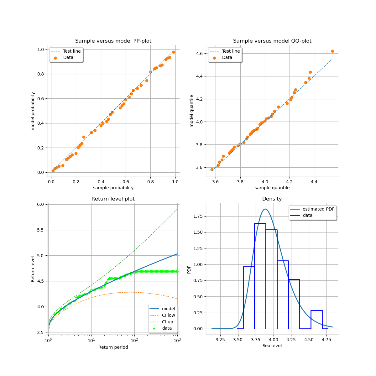
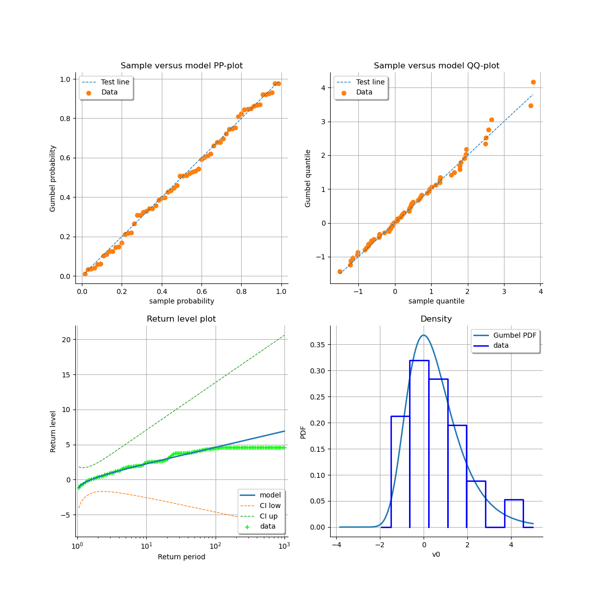
At last, we can validate the inference result thanks the 4 usual diagnostic plots.

validation = ot.GeneralizedExtremeValueValidation(result_LL, sample)
graph = validation.drawDiagnosticPlot()
view = otv.View(graph)

, Sample versus model PP-plot, Sample versus model QQ-plot, Return level plot, Density

Stationary GEV modeling via the profile log-likelihood function

Now, we use the profile log-likehood function rather than log-likehood function to estimate the parameters of the GEV.

result_PLL = factory.buildMethodOfXiProfileLikelihoodEstimator(sample)

The following graph allows one to get the profile log-likelihood plot. It also indicates the optimal value of $\xi$ , the maximum profile log-likelihood and the confidence interval for $\xi$ of order 0.95 (which is the default value).

order = 0.95
result_PLL.setConfidenceLevel(order)
view = otv.View(result_PLL.drawProfileLikelihoodFunction())

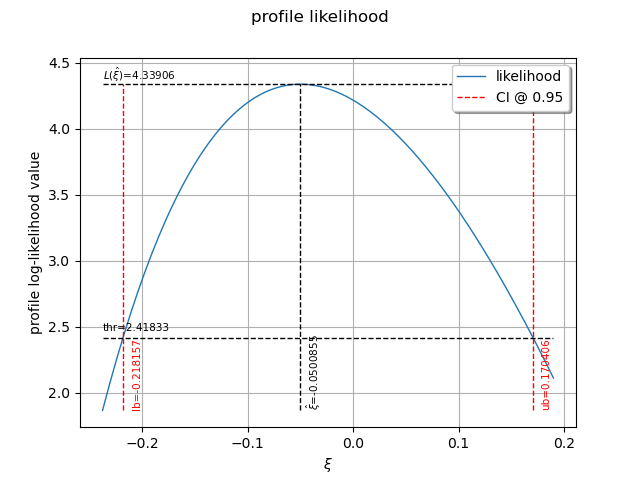
We can get the numerical values of the confidence interval: it appears to be a bit smaller with the interval obtained from the profile log-likelihood function than with the log-likelihood function. Note that if the order requested is too high, the confidence interval might not be calculated because one of its bound is out of the definition domain of the log-likelihood function.

try:
    print("Confidence interval for xi = ", result_PLL.getParameterConfidenceInterval())
except Exception as ex:
    print(type(ex))
    pass

Confidence interval for xi =  [-0.218157, 0.170406]

Return level estimate from the estimated stationary GEV

We estimate the $m$ -block return level $z_m$ : it is computed as a particular quantile of the GEV model estimated using the log-likelihood function. We just have to use the maximum log-likelihood estimator built in the previous section.

As the data are annual sea-levels, each block corresponds to one year: the 10-year return level corresponds to $m=10$ and the 100-year return level corresponds to $m=100$ .

The method also provides the asymptotic distribution of the estimator $\hat{z}_m$ .

zm_10 = factory.buildReturnLevelEstimator(result_LL, 10.0)
return_level_10 = zm_10.getMean()
print("Maximum log-likelihood function : ")
print(f"10-year return level = {return_level_10}")
return_level_ci10 = zm_10.computeBilateralConfidenceInterval(0.95)
print(f"CI = {return_level_ci10}")

zm_100 = factory.buildReturnLevelEstimator(result_LL, 100.0)
return_level_100 = zm_100.getMean()
print(f"100-year return level = {return_level_100}")
return_level_ci100 = zm_100.computeBilateralConfidenceInterval(0.95)
print(f"CI = {return_level_ci100}")

Maximum log-likelihood function :
10-year return level = [4.29619]
CI = [4.17405, 4.41834]
100-year return level = [4.68824]
CI = [4.28031, 5.09616]

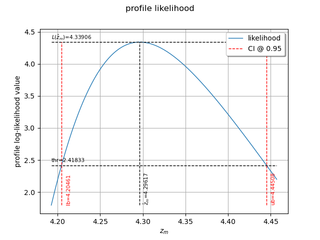
Return level estimate via the profile log-likelihood function of a stationary GEV

We can estimate the $m$ -block return level $z_m$ directly from the data using the profile likelihood with respect to $z_m$ .

result_zm_10_PLL = factory.buildReturnLevelProfileLikelihoodEstimator(sample, 10.0)
zm_10_PLL = result_zm_10_PLL.getParameter()
print(f"10-year return level (profile) = {zm_10_PLL}")

10-year return level (profile) = 4.296169941103285

We can get the confidence interval of $z_m$ : once more, it appears to be a bit smaller than the interval obtained from the log-likelihood function.

result_zm_10_PLL.setConfidenceLevel(0.95)
return_level_ci10 = result_zm_10_PLL.getParameterConfidenceInterval()
print("Maximum profile log-likelihood function : ")
print(f"CI={return_level_ci10}")

Maximum profile log-likelihood function :
CI=[4.20461, 4.44508]

We can also plot the profile log-likelihood function and get the confidence interval, the optimal value of $z_m$ and its confidence interval.

view = otv.View(result_zm_10_PLL.drawProfileLikelihoodFunction())

Non stationary GEV modeling via the log-likelihood function

Now, we want to see whether it is necessary to model the time dependence over the observation period.

We have to define the functional basis for each parameter of the GEV model. Even if we have the possibility to affect a time-varying model to each of the 3 parameters $(\mu, \sigma, \xi)$ , it is strongly recommended not to vary the parameter $\xi$ .

We suppose that $\mu$ is linear with time, and that the other parameters remain constant.

For numerical reasons, it is strongly recommended to normalize all the data as follows:

$\tau(t) = \dfrac{t-c}{d}$

where:

the CenterReduce method where $c = \dfrac{1}{n} \sum_{i=1}^n t_i$ is the mean time stamps and $d = \sqrt{\dfrac{1}{n} \sum_{i=1}^n (t_i-c)^2}$ is the standard deviation of the time stamps;
the MinMax method where $c = t_1$ is the initial time and $d = t_n-t_1$ the final time;
the None method where $c = 0$ and $d = 1$ : in that case, data are not normalized.

$\begin{align*} \mu(t) & = \beta_1 + \beta_2\tau(t) \\ \sigma(t) & = \beta_3 \\ \xi(t) & = \beta_4 \end{align*}$

constant = ot.SymbolicFunction(["t"], ["1.0"])
basis = ot.Basis([constant, ot.SymbolicFunction(["t"], ["t"])])
# basis for mu, sigma, xi
muIndices = [0, 1]  # linear
sigmaIndices = [0]  # stationary
xiIndices = [0]  # stationary

We need to get the time stamps (in years here).

timeStamps = data[:, 0]

We can now estimate the list of coefficients $\vect{\beta} = (\beta_1, \beta_2, \beta_3, \beta_4)$ using the log-likelihood of the data. We test the 3 normalizing methods and both initial points in order to evaluate their impact on the results. We can see that:

both normalization methods lead to the same result for $\beta_1$ , $\beta_3$ and $\beta_4$ (note that $\beta_2$ depends on the normalization function),
both initial points lead to the same result when the data have been normalized,
it is very important to normalize all the data: if not, the result strongly depends on the initial point and it differs from the result obtained with normalized data. The results are not optimal in that case since the associated log-likelihood are much smaller than those obtained with normalized data.

print("Linear mu(t) model: ")
for normMeth in ["MinMax", "CenterReduce", "None"]:
    for initPoint in ["Gumbel", "Static"]:
        print(f"normMeth = {normMeth}, initPoint = {initPoint}")
        # The ot.Function() is the identity function.
        result = factory.buildTimeVarying(
            sample,
            timeStamps,
            basis,
            muIndices,
            sigmaIndices,
            xiIndices,
            ot.Function(),
            ot.Function(),
            ot.Function(),
            initPoint,
            normMeth,
        )
        beta = result.getOptimalParameter()
        print(f"beta = {beta}")
        print(f"Max log-likelihood = {result.getLogLikelihood()}")

Linear mu(t) model:
normMeth = MinMax, initPoint = Gumbel
beta = [3.88617,-0.0226606,0.197965,-0.050304]
Max log-likelihood = 4.375105790428855
normMeth = MinMax, initPoint = Static
beta = [3.88616,-0.022621,0.197965,-0.0504251]
Max log-likelihood = 4.375106565819115
normMeth = CenterReduce, initPoint = Gumbel
beta = [3.87484,-0.00671465,0.197963,-0.0503351]
Max log-likelihood = 4.37510636082818
normMeth = CenterReduce, initPoint = Static
beta = [3.87484,-0.00671264,0.197968,-0.0503167]
Max log-likelihood = 4.375106107985937
normMeth = None, initPoint = Gumbel
beta = [3.89541,-1.63808e-05,0.197743,0.100071]
Max log-likelihood = 3.347363151272668
normMeth = None, initPoint = Static
beta = [3.87477,-3.43115e-10,0.198052,-0.0502339]
Max log-likelihood = 4.339057650029008

According to the previous results, we choose the MinMax normalization method and the Gumbel initial point. This initial point is cheaper than the Static one as it requires no optimization computation.

result_NonStatLL = factory.buildTimeVarying(
    sample, timeStamps, basis, muIndices, sigmaIndices, xiIndices
)
beta = result_NonStatLL.getOptimalParameter()
print(f"beta = {beta}")
print(f"mu(t) = {beta[0]:.4f} + {beta[1]:.4f} * tau")
print(f"sigma = {beta[2]:.4f}")
print(f"xi = {beta[3]:.4f}")

beta = [3.88617,-0.0226606,0.197965,-0.050304]
mu(t) = 3.8862 + -0.0227 * tau
sigma = 0.1980
xi = -0.0503

We get the asymptotic distribution of $\vect{\beta}$ to compute some confidence intervals of the estimates, for example of order $p = 0.95$ .

dist_beta = result_NonStatLL.getParameterDistribution()
confidence_level = 0.95
for i in range(beta.getSize()):
    lower_bound = dist_beta.getMarginal(i).computeQuantile((1 - confidence_level) / 2)[
        0
    ]
    upper_bound = dist_beta.getMarginal(i).computeQuantile((1 + confidence_level) / 2)[
        0
    ]
    print(
        "Conf interval for beta_"
        + str(i + 1)
        + " = ["
        + str(lower_bound)
        + "; "
        + str(upper_bound)
        + "]"
    )

Conf interval for beta_1 = [3.8732412530798044; 3.8990921585006806]
Conf interval for beta_2 = [-0.04478687551177846; -0.0005342704340991523]
Conf interval for beta_3 = [0.1921808327171997; 0.20374875413461713]
Conf interval for beta_4 = [-0.08320898064356753; -0.01739907207644617]

You can get the expression of the normalizing function $t \mapsto \tau(t)$ :

normFunc = result_NonStatLL.getNormalizationFunction()
print("Function tau(t): ", normFunc)
print("c = ", normFunc.getEvaluation().getImplementation().getCenter()[0])
print("1/d = ", normFunc.getEvaluation().getImplementation().getLinear()[0, 0])

Function tau(t):  class=LinearFunction name=Unnamed implementation=class=LinearEvaluation name=Unnamed center=[1923] constant=[0] linear=[[ 0.015625 ]]
c =  1923.0
1/d =  0.015625

You can get the function $t \mapsto \vect{\theta}(t)$ where $\vect{\theta}(t) = (\mu(t), \sigma(t), \xi(t))$ .

functionTheta = result_NonStatLL.getParameterFunction()

In order to compare different modelings, we get the optimal log-likelihood of the data for both stationary and non stationary models. The difference seems to be non significant enough, which means that the non stationary model does not really improve the quality of the modeling.

print("Max log-likelihood: ")
print("Stationary model =  ", result_LL.getLogLikelihood())
print("Non stationary linear mu(t) model =  ", result_NonStatLL.getLogLikelihood())

Max log-likelihood:
Stationary model =   4.339057644664945
Non stationary linear mu(t) model =   4.375105790428855

In order to draw some diagnostic plots similar to those drawn in the stationary case, we refer to the following result: if $Z_t$ is a non stationary GEV model parametrized by $(\mu(t), \sigma(t), \xi(t))$ , then the standardized variables $\hat{Z}_t$ defined by:

$\hat{Z}_t = \dfrac{1}{\xi(t)} \log \left[1+ \xi(t)\left( \dfrac{Z_t-\mu(t)}{\sigma(t)} \right)\right]$

have the standard Gumbel distribution which is the GEV model with $(\mu, \sigma, \xi) = (0, 1, 0)$ .

As a result, we can validate the inference result thanks the 4 usual diagnostic plots:

the probability-probability pot,
the quantile-quantile pot,
the return level plot,
the data histogram and the density of the fitted model.

using the transformed data compared to the Gumbel model. We can see that the adequation seems similar to the graph of the stationary model.

graph = result_NonStatLL.drawDiagnosticPlot()
view = otv.View(graph)

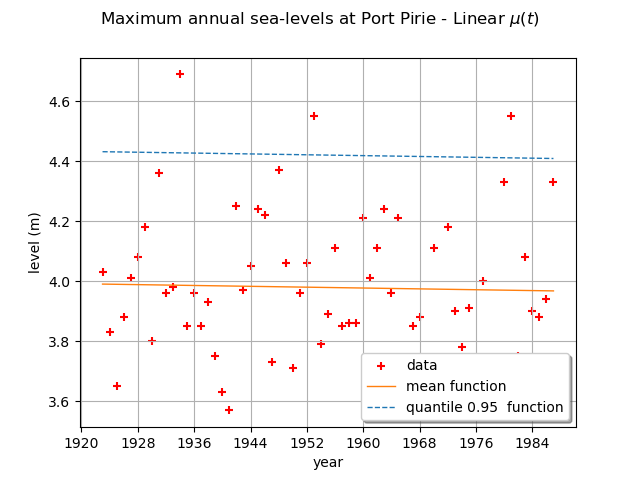
We can draw the mean function $t \mapsto \Expect{\mbox{GEV}(t)}$ . Be careful, it is not the function $t \mapsto \mu(t)$ . As a matter of fact, the mean is defined for $\xi <1$ only and in that case, for $\xi \neq 0$ , we have:

$\Expect{\mbox{GEV}(t)} = \mu(t) + \dfrac{\sigma(t)}{\xi(t)} (\Gamma(1-\xi(t))-1)$

and for $\xi = 0$ , we have:

$\Expect{\mbox{GEV}(t)} = \mu(t) + \sigma(t)\gamma$

where $\gamma$ is the Euler constant.

We can also draw the function $t \mapsto q_p(t)$ where $q_p(t)$ is the quantile of order $p$ of the GEV distribution at time $t$ . Here, $\mu(t)$ is a linear function and the other parameters are constant, so the mean and the quantile functions are also linear functions.

graph = ot.Graph(
    r"Maximum annual sea-levels at Port Pirie - Linear $\mu(t)$",
    "year",
    "level (m)",
    True,
    "",
)
graph.setIntegerXTick(True)
# data
cloud = ot.Cloud(data[:, :2])
cloud.setColor("red")
graph.add(cloud)
# mean function
meandata = [
    result_NonStatLL.getDistribution(t).getMean()[0] for t in data[:, 0].asPoint()
]
curve_meanPoints = ot.Curve(data[:, 0].asPoint(), meandata)
graph.add(curve_meanPoints)
# quantile function
graphQuantile = result_NonStatLL.drawQuantileFunction(0.95)
drawQuant = graphQuantile.getDrawable(0)
drawQuant = graphQuantile.getDrawable(0)
drawQuant.setLineStyle("dashed")
graph.add(drawQuant)
graph.setLegends(["data", "mean function", "quantile 0.95 function"])
graph.setLegendPosition("lower right")
view = otv.View(graph)

$Maximum annual sea-levels at Port Pirie - Linear $\mu(t)$$

At last, we can test the validity of the stationary model $\mathcal{M}_0$ relative to the model with time varying parameters $\mathcal{M}_1$ . The model $\mathcal{M}_0$ is parametrized by $(\beta_1, \beta_3, \beta_4)$ and the model $\mathcal{M}_1$ is parametrized by $(\beta_1, \beta_2, \beta_3, \beta_4)$ : so we have $\mathcal{M}_0 \subset \mathcal{M}_1$ .

We use the Likelihood Ratio test. The null hypothesis is the stationary model $\mathcal{M}_0$ . The Type I error $\alpha$ is taken equal to 0.05.

This test confirms that there is no evidence of a linear trend for $\mu$ .

llh_LL = result_LL.getLogLikelihood()
llh_NonStatLL = result_NonStatLL.getLogLikelihood()
modelM0_Nb_param = 3
modelM1_Nb_param = 4
resultLikRatioTest = ot.HypothesisTest.LikelihoodRatioTest(
    modelM0_Nb_param, llh_LL, modelM1_Nb_param, llh_NonStatLL, 0.05
)
accepted = resultLikRatioTest.getBinaryQualityMeasure()
print(
    f"Hypothesis H0 (stationary model) vs H1 (linear mu(t) model):  accepted ? = {accepted}"
)

Hypothesis H0 (stationary model) vs H1 (linear mu(t) model):  accepted ? = True

We detail the statistics of the Likelihood Ratio test: the deviance statistics $\mathcal{D}_p$ follows a $\chi^2_1$ distribution. The model $\mathcal{M}_0$ is rejected if the deviance statistics estimated on the data is greater than the threshold $c_{\alpha}$ or if the p-value is less than the Type I error $\alpha = 0.05$ .

print(f"Dp={resultLikRatioTest.getStatistic():.2f}")
print(f"alpha={resultLikRatioTest.getThreshold():.2f}")
print(f"p-value={resultLikRatioTest.getPValue():.2f}")

Dp=0.07
alpha=0.05
p-value=0.79

otv.View.ShowAll()

OpenTURNS

An Open source initiative for the Treatment of Uncertainties, Risks'N Statistics

Previous topic

Next topic

This Page

Estimate a GEV on the Port Pirie sea-levels data¶