Note

Go to the end to download the full example code.

Estimate a GPD on the daily rainfall data¶

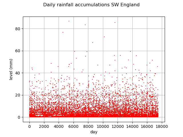
In this example, we illustrate various techniques of extreme value modeling applied to the daily rainfall accumulations in south-west England, over the period 1914-1962. Readers should refer to [coles2001] to get more details.

We illustrate techniques to:

estimate a stationary and a non stationary GPD,
estimate a return level,

using:

the log-likelihood function,
the profile log-likelihood function.

import openturns as ot
import openturns.experimental as otexp
import openturns.viewer as otv
from openturns.usecases import coles

First, we load the Rain dataset. We start by looking at it through time.

dataRain = coles.Coles().rain
print(dataRain[:10])
graph = ot.Graph(
    "Daily rainfall accumulations SW England", "day", "level (mm)", True, ""
)
days = ot.Sample([[i] for i in range(len(dataRain))])
cloud = ot.Cloud(days, dataRain)
cloud.setColor("red")
cloud.setPointStyle(",")
graph.add(cloud)
graph.setIntegerXTick(True)
view = otv.View(graph)

    [ x   ]
: [ 0   ]
: [ 2.3 ]
: [ 1.3 ]
: [ 6.9 ]
: [ 4.6 ]
: [ 0   ]
: [ 1   ]
: [ 1.5 ]
: [ 1.8 ]
: [ 1.8 ]

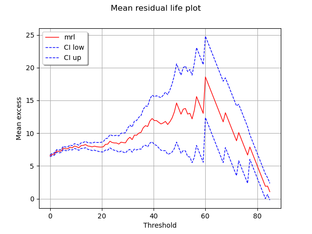
In order to select a threshold upon which the GPD model will be fitted, we draw the mean residual life plot with approximate $95\%$ confidence interval. It appears that the graph is linear from the threshold around $u=30$ . Then, it decays sharply although with a linear trend. We should be tempted to choose $u=60$ but there are only 6 exceedances of the threshold $u=60$ . So it is not enough to make meaningful inferences. Moreover, the graph is not reliable for large values of $u$ due to the limited amount of data on which the estimate and the confidence interval are based. For all these reasons, it appears preferable to chose $u=30$ .

factory = ot.GeneralizedParetoFactory()
graph = factory.drawMeanResidualLife(dataRain)
view = otv.View(graph)

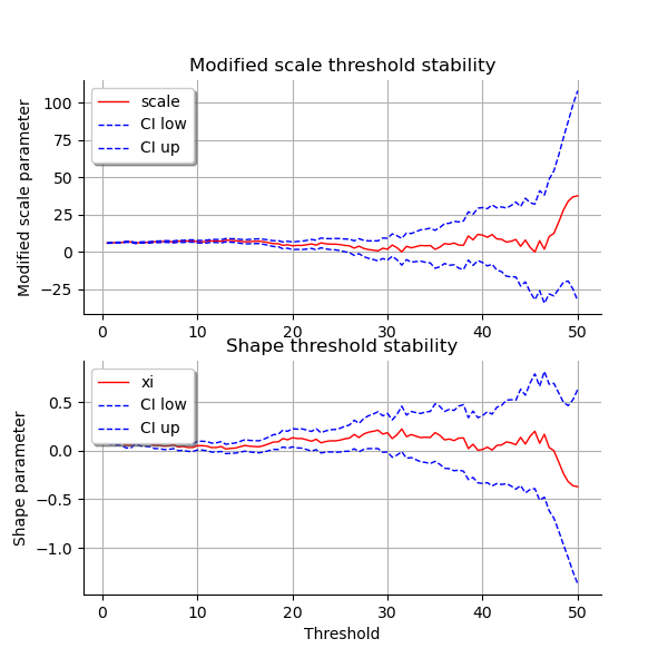
To support that choice, we draw the parameter stability plots. We see that the perturbations appear small relatively to sampling errors. We can see that the change in pattern observed in the mean residual life plot is still apparent here for high thresholds. Hence, we choose the threshold $u=30$ .

u_range = ot.Interval(0.5, 50.0)
graph = factory.drawParameterThresholdStability(dataRain, u_range)
view = otv.View(graph, figure_kw={"figsize": (6.0, 6.0)})

, Modified scale threshold stability, Shape threshold stability

Stationary GPD modeling via the log-likelihood function

We first assume that the dependence through time is negligible, so we first model the data as independent observations over the observation period.

We consider the model $\mathcal{M}_0$ defined by:

$\begin{align*} \sigma(t) & = \sigma\\ \xi(t) & = \xi \end{align*}$

We estimate the parameters of the GPD distribution by maximizing the log-likelihood of the data for the selecte threshold $u=30$ .

u = 30
result_LL = factory.buildMethodOfLikelihoodMaximizationEstimator(dataRain, u)

We get the fitted GPD and its parameters of $(\hat{\sigma}, \hat{\xi}, u)$ .

fitted_GPD = result_LL.getDistribution()
desc = fitted_GPD.getParameterDescription()
param = fitted_GPD.getParameter()
print(", ".join([f"{p}: {value:.3f}" for p, value in zip(desc, param)]))
print("log-likelihood = ", result_LL.getLogLikelihood())

sigma: 7.446, xi: 0.184, u: 30.000
log-likelihood =  -485.0937375341342

We get the asymptotic distribution of the estimator $(\hat{\mu}, \hat{\sigma}, \hat{\xi})$ . In that case, the asymptotic distribution is normal.

parameterEstimate = result_LL.getParameterDistribution()
print("Asymptotic distribution of the estimator : ")
print(parameterEstimate)

Asymptotic distribution of the estimator :
BlockIndependentDistribution(Normal(mu = [7.44573,0.184112], sigma = [0.959381,0.101172], R = [[  1        -0.675368 ]
 [ -0.675368  1        ]]), Dirac(point = [30]))

We get the covariance matrix and the standard deviation of $(\hat{\sigma}, \hat{\xi}, \hat{\xi})$ .

print("Cov matrix = \n", parameterEstimate.getCovariance())
print("Standard dev = ", parameterEstimate.getStandardDeviation())

Cov matrix =
 [[  0.920412  -0.0655531  0         ]
 [ -0.0655531  0.0102358  0         ]
 [  0          0          0         ]]
Standard dev =  [0.959381,0.101172,0]

We get the marginal confidence intervals of order 0.95.

order = 0.95
for i in range(2):  # exclude u parameter (fixed)
    ci = parameterEstimate.getMarginal(i).computeBilateralConfidenceInterval(order)
    print(desc[i] + ":", ci)

sigma: [5.56538, 9.32608]
xi: [-0.0141821, 0.382406]

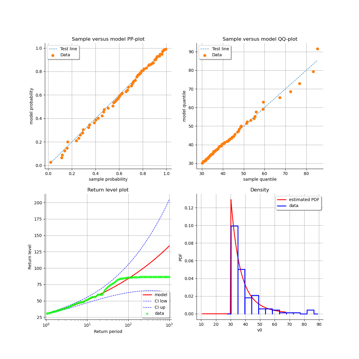
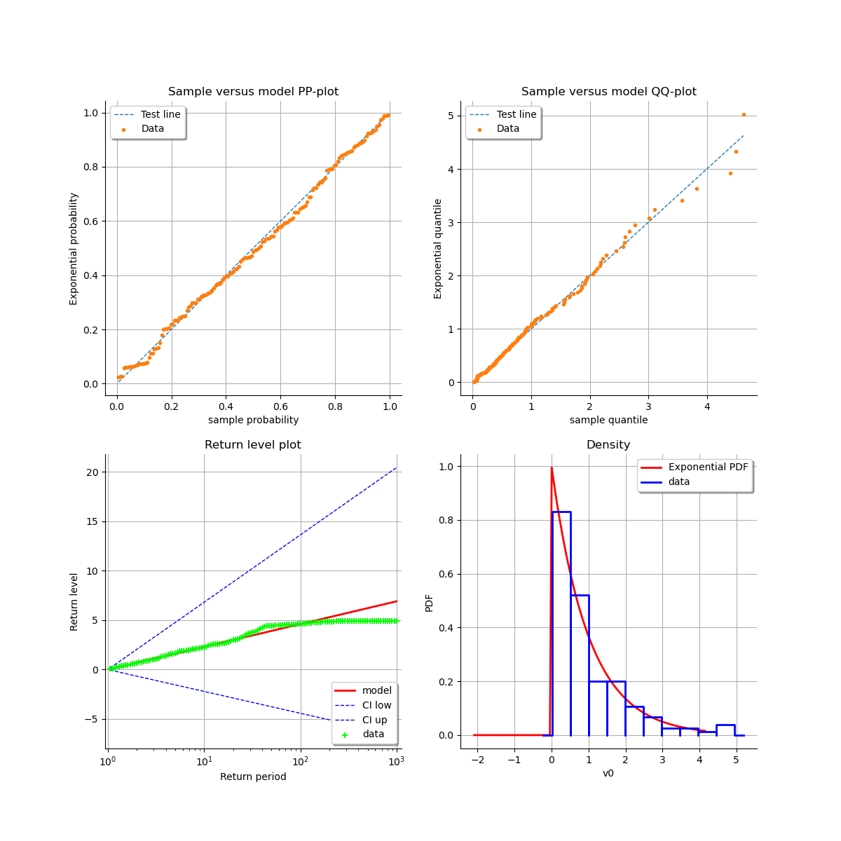
At last, we can validate the inference result thanks to the 4 usual diagnostic plots:

the probability-probability pot,
the quantile-quantile pot,
the return level plot,
the data histogram and the density of the fitted model.

validation = otexp.GeneralizedParetoValidation(result_LL, dataRain)
graph = validation.drawDiagnosticPlot()
view = otv.View(graph)

, Sample versus model PP-plot, Sample versus model QQ-plot, Return level plot, Density

Stationary GPD modeling via the profile log-likelihood function

Now, we use the profile log-likehood function with respect to the $\xi$ parameter rather than log-likehood function to estimate the parameters of the GPD.

result_PLL = factory.buildMethodOfXiProfileLikelihoodEstimator(dataRain, u)

The following graph allows one to get the profile log-likelihood plot. It also indicates the optimal value of $\xi$ , the maximum profile log-likelihood and the confidence interval for $\xi$ of order 0.95 (which is the default value).

order = 0.95
result_PLL.setConfidenceLevel(order)
view = otv.View(result_PLL.drawProfileLikelihoodFunction())

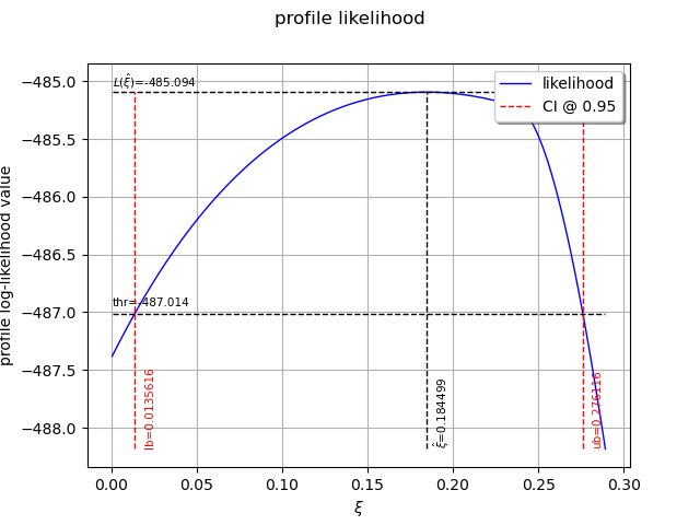
We can get the numerical values of the confidence interval: it appears to be a bit smaller with the interval obtained from the profile log-likelihood function than with the log-likelihood function. Note that if the order requested is too high, the confidence interval might not be calculated because one of its bound is out of the definition domain of the log-likelihood function.

try:
    print("Confidence interval for xi = ", result_PLL.getParameterConfidenceInterval())
except Exception as ex:
    print(type(ex))
    pass

Confidence interval for xi =  [0.0135616, 0.276116]

Return level estimate from the estimated stationary GPD

We evaluate the $T$ -year return level which corresponds to the $m$ -observation return level, where $m = T*n_y$ with $n_y$ the number of observations per year. Here, we have daily observations, hence $n_y = 365$ . As we assumed that the observations were independent, the extremal index is $\theta=1$ which is the default value.

The method also provides the asymptotic distribution of the estimator $\hat{z}_m$ .

ny = 365
T10 = 10
zm_10 = factory.buildReturnLevelEstimator(result_LL, dataRain, T10 * ny)
return_level_10 = zm_10.getMean()
print("Maximum log-likelihood function : ")
print(f"10-year return level = {return_level_10}")
return_level_ci10 = zm_10.computeBilateralConfidenceInterval(0.95)
print(f"CI = {return_level_ci10}")

T100 = 100
zm_100 = factory.buildReturnLevelEstimator(result_LL, dataRain, T100 * ny)
return_level_100 = zm_100.getMean()
print(f"100-year return level = {return_level_100}")
return_level_ci100 = zm_100.computeBilateralConfidenceInterval(0.95)
print(f"CI = {return_level_ci100}")

Maximum log-likelihood function :
10-year return level = [65.9517]
CI = [55.6696, 76.2339]
100-year return level = [106.284]
CI = [65.4932, 147.075]

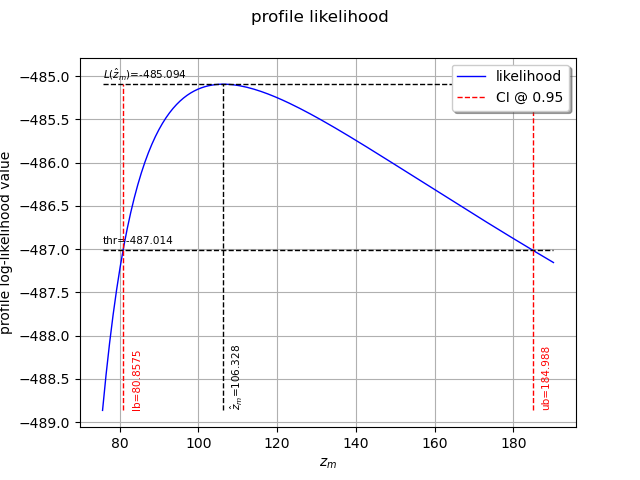
Return level estimate via the profile log-likelihood function of a stationary GPD

We can estimate the $m$ -observation return level $z_m$ directly from the data using the profile likelihood with respect to $z_m$ .

result_zm_100_PLL = factory.buildReturnLevelProfileLikelihoodEstimator(
    dataRain, u, T100 * ny
)
zm_100_PLL = result_zm_100_PLL.getParameter()
print(f"100-year return level (profile) = {zm_100_PLL}")

100-year return level (profile) = 106.32802943042479

We can get the confidence interval of $z_m$ : once more, it appears to be a bit smaller than the interval obtained from the log-likelihood function.

result_zm_100_PLL.setConfidenceLevel(0.95)
return_level_ci100 = result_zm_100_PLL.getParameterConfidenceInterval()
print("Maximum profile log-likelihood function : ")
print(f"CI={return_level_ci100}")

Maximum profile log-likelihood function :
CI=[80.8575, 184.988]

We can also plot the profile log-likelihood function and get the confidence interval, the optimal value of $z_m$ and its confidence interval.

view = otv.View(result_zm_100_PLL.drawProfileLikelihoodFunction())

Non stationary GPD modeling via the log-likelihood function

Now, we want to check whether it is necessary to model the time dependency over the observation period.

We have to define the functional basis for each parameter of the GPD model. Even if we have the possibility to affect a time-varying model to each of the 2 parameters $(\sigma, \xi)$ , it is strongly recommended not to vary the shape parameter $\xi$ .

We suppose that $\sigma$ is linear with time, and that the other parameters remain constant.

For numerical reasons, it is strongly recommended to normalize all the data as follows:

$\tau(t) = \dfrac{t-c}{d}$

where:

the CenterReduce method where $c = \dfrac{1}{n} \sum_{i=1}^n t_i$ is the mean time stamps and $d = \sqrt{\dfrac{1}{n} \sum_{i=1}^n (t_i-c)^2}$ is the standard deviation of the time stamps;
the MinMax method where $c = t_1$ is the initial time and $d = t_n-t_1$ the final time. This method is the default one;
the None method where $c = 0$ and $d = 1$ : in that case, data are not normalized.

We consider the model $\mathcal{M}_1$ defined by:

$\begin{align*} \sigma(t) & = \beta_1 + \beta_2\tau(t) \\ \xi(t) & = \beta_3 \end{align*}$

constant = ot.SymbolicFunction(["t"], ["1.0"])
basis = ot.Basis([ot.SymbolicFunction(["t"], ["t"]), constant])
# basis for mu, sigma, xi
sigmaIndices = [0, 1]  # linear
xiIndices = [1]  # stationary

We need to get the time stamps (in days here).

timeStamps = ot.Sample([[i + 1] for i in range(len(dataRain))])

We can now estimate the list of coefficients $\vect{\beta} = (\beta_1, \beta_2, \beta_3)$ using the log-likelihood of the data.

result_NonStatLL = factory.buildTimeVarying(
    dataRain, u, timeStamps, basis, sigmaIndices, xiIndices
)
beta = result_NonStatLL.getOptimalParameter()
print(f"beta = {beta}")
print(f"sigma(t) = {beta[1]:.4f} * tau(t) + {beta[0]:.4f}")
print(f"xi = {beta[2]:.4f}")
print(f"Max log-likelihood = {result_NonStatLL.getLogLikelihood()}")

beta = [0.882226,7.01759,0.18162]
sigma(t) = 7.0176 * tau(t) + 0.8822
xi = 0.1816
Max log-likelihood = -484.8061273999882

We get the asymptotic distribution of $\vect{\beta}$ to compute some confidence intervals of the estimates, for example of order $p = 0.95$ .

dist_beta = result_NonStatLL.getParameterDistribution()
confidence_level = 0.95
for i in range(beta.getSize()):
    lower_bound = dist_beta.getMarginal(i).computeQuantile((1 - confidence_level) / 2)[
        0
    ]
    upper_bound = dist_beta.getMarginal(i).computeQuantile((1 + confidence_level) / 2)[
        0
    ]
    print(
        "Conf interval for beta_"
        + str(i + 1)
        + " = ["
        + str(lower_bound)
        + "; "
        + str(upper_bound)
        + "]"
    )

Conf interval for beta_1 = [0.8822255895863612; 0.8822255895863612]
Conf interval for beta_2 = [7.017592488770449; 7.017592488770449]
Conf interval for beta_3 = [0.18161982259931925; 0.18161982259931925]

You can get the expression of the normalizing function $t \mapsto \tau(t)$ :

normFunc = result_NonStatLL.getNormalizationFunction()
print("Function tau(t): ", normFunc)
print("c = ", normFunc.getEvaluation().getImplementation().getCenter()[0])
print("1/d = ", normFunc.getEvaluation().getImplementation().getLinear()[0, 0])

Function tau(t):  class=LinearFunction name=Unnamed implementation=class=LinearEvaluation name=Unnamed center=[1] constant=[0] linear=[[ 5.70451e-05 ]]
c =  1.0
1/d =  5.7045065601825445e-05

You can get the function $t \mapsto \vect{\theta}(t)$ where $\vect{\theta}(t) = (\sigma(t), \xi(t))$ .

functionTheta = result_NonStatLL.getParameterFunction()

In order to compare different modelings, we get the optimal log-likelihood of the data for both stationary and non stationary models. The difference seems to be non significant enough, which means that the non stationary model does not really improve the quality of the modeling.

print("Max log-likelihood: ")
print("Stationary model =  ", result_LL.getLogLikelihood())
print("Non stationary linear sigma(t) model =  ", result_NonStatLL.getLogLikelihood())

Max log-likelihood:
Stationary model =   -485.0937375341342
Non stationary linear sigma(t) model =   -484.8061273999882

In order to draw some diagnostic plots similar to those drawn in the stationary case, we refer to the following result: if $Y_t$ is a non stationary GPD model parametrized by $(\sigma(t), \xi(t), u)$ , then the standardized variables $\hat{Y}_t$ defined by:

$\hat{Y}_t = \dfrac{1}{\xi(t)} \log \left[1+ \xi(t)\left( \dfrac{Y_t-u}{\sigma(t)} \right)\right]$

have the Exponential distribution which is the GPD model with $(\sigma, \xi, u) = (1, 0, 0)$ .

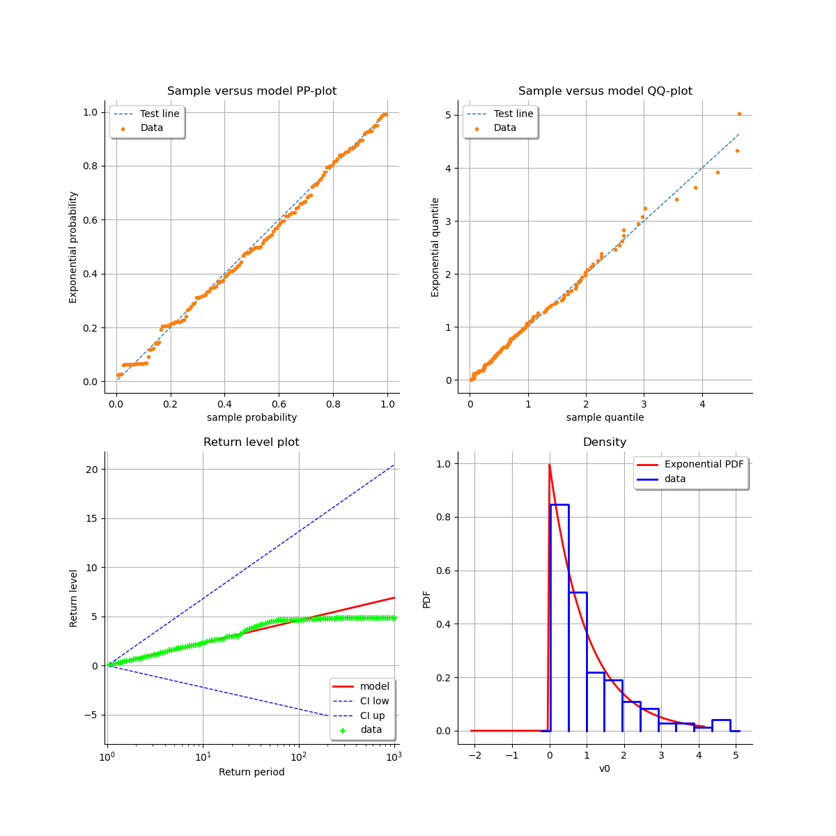
As a result, we can validate the inference result thanks the 4 usual diagnostic plots:

the probability-probability pot,
the quantile-quantile pot,
the return level plot,
the data histogram and the density of the fitted model.

using the transformed data compared to the Exponential model. We can see that the adequation seems similar to the graph of the stationary model.

graph = result_NonStatLL.drawDiagnosticPlot()
view = otv.View(graph)

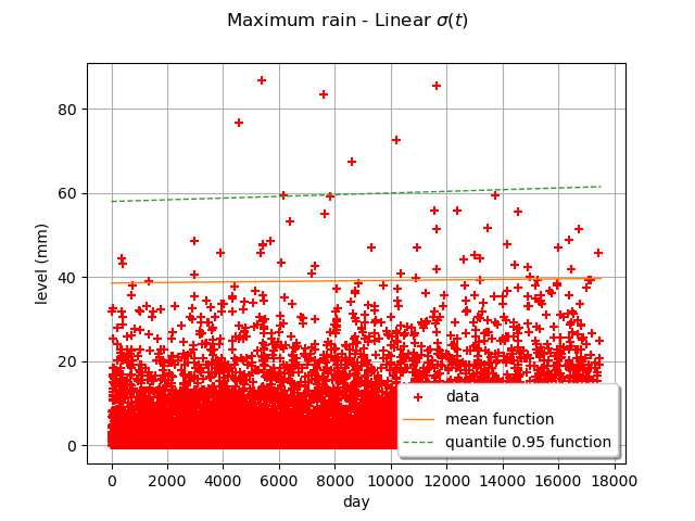
We can draw the mean function $t \mapsto \Expect{\mbox{GPD}(t)}$ , defined for $\xi <1$ only:

$\Expect{\mbox{GPD}(t)} = u + \dfrac{\sigma(t)}{1 - \xi(t)}$

We can also draw the function $t \mapsto q_p(t)$ where $q_p(t)$ is the quantile of order $p$ of the GPD distribution at time $t$ . Here, $\sigma(t)$ is a linear function and the other parameters are constant, so the mean and the quantile functions are also linear functions.

graph = ot.Graph(
    r"Maximum rain - Linear $\sigma(t)$",
    "day",
    "level (mm)",
    True,
    "",
)
graph.setIntegerXTick(True)
# data
cloud = ot.Cloud(timeStamps, dataRain)
cloud.setColor("red")
graph.add(cloud)
# mean function
meandata = [
    result_NonStatLL.getDistribution(t).getMean()[0] for t in timeStamps.asPoint()
]
curve_meanPoints = ot.Curve(timeStamps.asPoint(), meandata)
graph.add(curve_meanPoints)
# quantile function
graphQuantile = result_NonStatLL.drawQuantileFunction(0.95)
drawQuant = graphQuantile.getDrawable(0)
drawQuant = graphQuantile.getDrawable(0)
drawQuant.setLineStyle("dashed")
graph.add(drawQuant)
graph.setLegends(["data", "mean function", "quantile 0.95 function"])
graph.setLegendPosition("lower right")
view = otv.View(graph)

$Maximum rain - Linear $\sigma(t)$$

At last, we can test the validity of the stationary model $\mathcal{M}_0$ relative to the model with time varying parameters $\mathcal{M}_1$ . The model $\mathcal{M}_0$ is parametrized by $(\beta_1, \beta_3)$ and the model $\mathcal{M}_1$ is parametrized by $(\beta_1, \beta_2, \beta_3)$ : so we have $\mathcal{M}_0 \subset \mathcal{M}_1$ .

We use the Likelihood Ratio test. The null hypothesis is the stationary model $\mathcal{M}_0$ . The Type I error $\alpha$ is taken equal to 0.05.

This test confirms that there is no evidence of a linear trend for $\mu$ .

llh_LL = result_LL.getLogLikelihood()
llh_NonStatLL = result_NonStatLL.getLogLikelihood()
modelM0_Nb_param = 2
modelM1_Nb_param = 3
resultLikRatioTest = ot.HypothesisTest.LikelihoodRatioTest(
    modelM0_Nb_param, llh_LL, modelM1_Nb_param, llh_NonStatLL, 0.05
)
accepted = resultLikRatioTest.getBinaryQualityMeasure()
print(
    f"Hypothesis H0 (stationary model) vs H1 (linear mu(t) model):  accepted ? = {accepted}"
)

Hypothesis H0 (stationary model) vs H1 (linear mu(t) model):  accepted ? = True

We detail the statistics of the Likelihood Ratio test: the deviance statistics $\mathcal{D}_p$ follows a $\chi^2_1$ distribution. The model $\mathcal{M}_0$ is rejected if the deviance statistics estimated on the data is greater than the threshold $c_{\alpha}$ or if the p-value is less than the Type I error $\alpha = 0.05$ .

print(f"Dp={resultLikRatioTest.getStatistic():.2f}")
print(f"alpha={resultLikRatioTest.getThreshold():.2f}")
print(f"p-value={resultLikRatioTest.getPValue():.2f}")

Dp=0.58
alpha=0.05
p-value=0.45

We can test a linear trend in the log-scale parameter for $\sigma(t)$ :

$\begin{align*} \sigma(t) & = exp(\beta_1 + \beta_2\tau(t)) \\ \xi(t) & = \beta_3 \end{align*}$

sigmaLink = ot.SymbolicFunction("x", "exp(x)")
result_NonStatLL_Link = factory.buildTimeVarying(
    dataRain, u, timeStamps, basis, sigmaIndices, xiIndices, sigmaLink
)
beta = result_NonStatLL_Link.getOptimalParameter()
print(f"beta = {beta}")
print(f"sigma(t) = exp({beta[1]:.4f} * tau(t) + {beta[0]:.4f})")
print(f"xi = {beta[2]:.4f}")
print(f"Max log-likelihood = {result_NonStatLL.getLogLikelihood()}")

# %
# The maximized log-likelihood we obtain with the log-linear model is very similar
# to the one we obtained with the linear model. Hence, there is no evidence of a time trend.
# We draw the diagnostic plots which are similar to the previous ones.
graph = result_NonStatLL_Link.drawDiagnosticPlot()
view = otv.View(graph)

beta = [0.343272,1.80443,0.197766]
sigma(t) = exp(1.8044 * tau(t) + 0.3433)
xi = 0.1978
Max log-likelihood = -484.8061273999882

otv.View.ShowAll()

Total running time of the script: (0 minutes 25.036 seconds)

OpenTURNS

An Open source initiative for the Treatment of Uncertainties, Risks'N Statistics

Previous topic

Next topic

This Page

Estimate a GPD on the daily rainfall data¶