Viscous free fall: metamodel of a field function

In this example, we present how to create the metamodel of a field function. This examples considers the free fall model. We create the metamodel automatically using openturns.experimental.PointToFieldFunctionalChaosAlgorithm and then also with a manual approach: We first compute the Karhunen-Loève decomposition of a sample of trajectories. Then we create a create a polynomial chaos which takes the inputs and returns the KL decomposition modes as outputs. Finally, we create a metamodel by combining the KL decomposition and the polynomial chaos.

Define the model

import openturns as ot
import openturns.experimental as otexp
import openturns.viewer as otv
from openturns.usecases import viscous_free_fall

ot.Log.Show(ot.Log.NONE)

Load the viscous free fall example.

vff = viscous_free_fall.ViscousFreeFall()
distribution = vff.distribution
model = vff.model

Generate a training sample.

size = 2000
ot.RandomGenerator.SetSeed(0)
inputSample = distribution.getSample(size)
outputSample = model(inputSample)

Compute the global metamodel

algo = otexp.PointToFieldFunctionalChaosAlgorithm(
    inputSample, outputSample, distribution
)
algo.run()
result = algo.getResult()
metaModel = result.getPointToFieldMetaModel()

Validate the metamodel

Create a validation sample.

size = 10
validationInputSample = distribution.getSample(size)
validationOutputSample = model(validationInputSample)

graph = validationOutputSample.drawMarginal(0)
graph.setColors(["red"])
graph2 = metaModel(validationInputSample).drawMarginal(0)
graph2.setColors(["blue"])
graph.add(graph2)
graph.setTitle("Model/metamodel comparison")
graph.setXTitle(r"$t$")
graph.setYTitle(r"$z$")
view = otv.View(graph)

We see that the blue trajectories (i.e. the metamodel) are close to the red trajectories (i.e. the validation sample). This shows that the metamodel is quite accurate. However, we observe that the trajectory singularity that occurs when the object touches the ground (i.e. when is equal to zero), makes the metamodel less accurate.

Sensitivity analysis

Compute the sensitivity indices

sensitivity = otexp.FieldFunctionalChaosSobolIndices(result)
s1 = sensitivity.getFirstOrderIndices()
st = sensitivity.getTotalOrderIndices()

We can notice that v0 and m are the most influencial parameters and that there are almost no interactions (total indices being close to first order indices)

print(s1, st)

[0.000544767,0.761005,0.229523,0.00219036] [0.00296842,0.76534,0.23269,0.00591793]

Draw the sensitivity indices

graph = sensitivity.draw()
view = otv.View(graph)

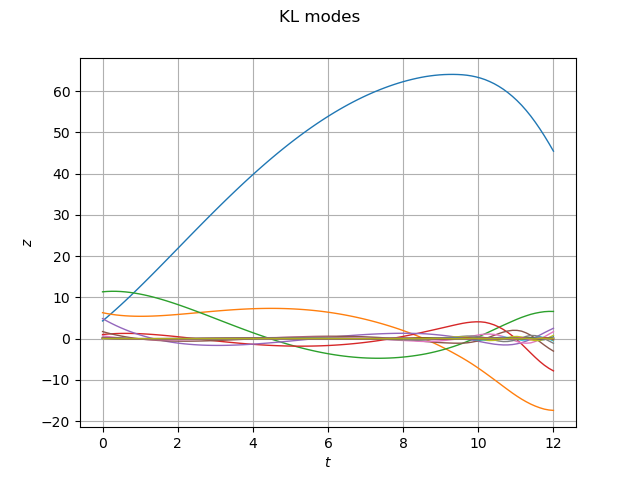
Manual approach

Step 1: compute the KL decomposition of the output

algo = ot.KarhunenLoeveSVDAlgorithm(outputSample, 1.0e-6)
algo.run()
klResult = algo.getResult()
scaledModes = klResult.getScaledModesAsProcessSample()

graph = scaledModes.drawMarginal(0)
graph.setTitle("KL modes")
graph.setXTitle(r"$t$")
graph.setYTitle(r"$z$")
view = otv.View(graph)

We create the lifting function which takes coefficients of the K.-L. modes as inputs and returns the trajectories.

klLiftingFunction = ot.KarhunenLoeveLifting(klResult)

The project method computes the projection of the output sample (i.e. the trajectories) onto the K.-L. modes.

outputSampleChaos = klResult.project(outputSample)

step 2: compute the metamodel of the KL modes

# We create a polynomial chaos metamodel which takes the input sample and returns the K.-L. modes.
algo = ot.FunctionalChaosAlgorithm(inputSample, outputSampleChaos, distribution)
algo.run()
chaosMetamodel = algo.getResult().getMetaModel()

The final metamodel is a composition of the KL lifting function and the polynomial chaos metamodel. We combine these two functions using the PointToFieldConnection class.

metaModel = ot.PointToFieldConnection(klLiftingFunction, chaosMetamodel)

Reset ResourceMap

ot.ResourceMap.Reload()

otv.View.ShowAll()