Note

Go to the end to download the full example code.

Compute leave-one-out error of a polynomial chaos expansion¶

Introduction¶

In this example, we compute the design matrix of a polynomial chaos expansion using the DesignProxy class. Then we compute the analytical leave-one-out error using the diagonal of the projection matrix. To do this, we use equations from [blatman2009] page 85 (see also [blatman2011]). In this advanced example, we use the DesignProxy and QRMethod low level classes. A naive implementation of this method is presented in Polynomial chaos expansion cross-validation using K-Fold cross-validation.

The design matrix¶

In this section, we analyze why the DesignProxy is linked to the classical linear least squares regression problem. Let $n$ be the number of observations and $m$ be the number of coefficients of the linear model. Let $D \in \mathbb{R}^{n \times m}$ be the design matrix, i.e. the matrix that produces the predictions of the linear regression model from the coefficients:

$\hat{\vect{y}} = D \vect{a}$

where $\vect{a} \in \mathbb{R}^m$ is the vector of coefficients, $\hat{y} \in \mathbb{R}^n$ is the vector of predictions. The linear least squares problem is:

$\operatorname{argmin}_{\vect{a} \in \mathbb{R}^m} \left\| D \vect{a} - \vect{y} \right\|_2^2.$

The solution is given by the normal equations, i.e. the vector of coefficients is the solution of the following linear system of equations:

$G \vect{a} = D^T \vect{y}$

where $G \in \Rset^{n \times n}$ is the Gram matrix:

G := D^T D.

The hat matrix is the projection matrix defined by:

$H := D \left(D^T D\right)^{-1} D^T.$

The hat matrix puts a hat to the vector of observations to produce the vector of predictions of the linear model:

$\hat{\vect{y}} = H \vect{y}$

To solve a linear least squares problem, we need to evaluate the design matrix $D$ , which is the primary goal of the DesignProxy class. Let us present some examples of situations where the design matrix is required.

When we use the QR decomposition, we actually do not need to evaluate it in our script: the QRMethod class knows how to compute the solution without evaluating the Gram matrix $D^T D$ .
We may need the inverse Gram matrix $\left(D^T D\right)^{-1}$ sometimes, for example when we want to create a D-optimal design.
Finally, when we want to compute the analytical leave-one-out error, we need to compute the diagonal of the projection matrix $H$ .

For all these purposes, the DesignProxy is the tool.

The leave-one-out error¶

In this section, we show that the leave-one-error of a regression problem can be computed using an analytical formula which depends on the hat matrix $H$ . We consider the physical model:

$y = g(\vect{x})$

where $\vect{x} \in \Rset^{n_X}$ is the input and $y \in \Rset$ is the output. Consider the problem of approximating the physical model $g$ by the linear model:

$\hat{y} := \tilde{g}(\vect{x}) = \sum_{k = 1}^m a_k \psi_k(\vect{x})$

for any $\vect{x} \in \Rset^{n_X}$ where $\{\psi_k : \Rset^{n_X} \rightarrow \Rset\}_{k = 1, \ldots, m}$ are the basis functions and $\vect{a} \in \Rset^m$ is a vector of parameters. The mean squared error is ([blatman2009] eq. 4.23 page 83):

$\operatorname{MSE}\left(\tilde{g}\right) = \mathbb{E}_{\vect{X}}\left[\left(g\left(\vect{X}\right) - \tilde{g}\left(\vect{X}\right) \right)^2 \right]$

The leave-one-out error is an estimator of the mean squared error. Let:

$\cD = \{\vect{x}^{(1)}, \ldots, \vect{x}^{(n)} \in \Rset^{n_X}\}$

be independent observations of the input random vector $\vect{X}$ and let $\{y^{(1)}, \ldots, y^{(n)} \in \Rset^{n_X}\}$ be the corresponding observations of the output of the physical model:

$y^{(j)} = g\left(\vect{x}^{(j)}\right)$

for $j = 1, ..., n$ . Let $\vect{y} \in \Rset^n$ be the vector of observations:

$\vect{y} = (y^{(1)}, \ldots, y^{(n)})^T.$

Consider the following set of inputs, let aside the $j$ -th input:

$\cD^{(-j)} := \left\{\vect{x}^{(1)}, \ldots, \vect{x}^{(j - 1)}, \vect{x}^{(j + 1)}, \ldots, \vect{x}^{(n)}\right\}$

for $j \in \{1, ..., n\}$ . Let $\vect{y}^{(-j)} \in \Rset^{n - 1}$ be the vector of observations, let aside the $j$ -th observation:

$\vect{y}^{(-j)} = (y^{(1)}, \ldots, y^{(j - 1)}, y^{(j + 1)}, \ldots, y^{(n)})^T$

for $j \in \{1, ..., n\}$ . Let $\tilde{g}^{(-j)}$ the metamodel built on the data set $\left(\cD^{(-j)}, \vect{y}^{(-j)}\right)$ . The leave-one-out error is:

$\widehat{\operatorname{MSE}}_{LOO}\left(\tilde{g}\right) = \frac{1}{n} \sum_{j = 1}^n \left(g\left(\vect{x}^{(j)}\right) - \tilde{g}^{(-j)}\left(\vect{x}^{(j)}\right)\right)^2$

The leave-one-out error is sometimes referred to as predicted residual sum of squares (PRESS) or jacknife error. In the next section, we show how this estimator can be computed analytically, using the hat matrix.

The analytical leave-one-out error¶

One limitation of the previous equation is that we must train $n$ different surrogate models, which can be long in some situations. To overcome this limitation, we can use the following equations. Let $\boldsymbol{\Psi} \in \Rset^{n \times m}$ design matrix ([blatman2009] eq. 4.32 page 85):

$\boldsymbol{\Psi}_{jk} = \psi_k\left(\vect{x}^{(j)}\right)$

for $j = 1, ..., n$ and $k = 1, ..., m$ . The matrix $\boldsymbol{\Psi}$ is mathematically equal to the $D$ matrix presented earlier in the present document. Let $H \in \Rset^{n \times n}$ be the projection matrix:

$H = \boldsymbol{\Psi} \left(\boldsymbol{\Psi}^T \boldsymbol{\Psi}\right) \boldsymbol{\Psi}^T.$

It can be proved that ([blatman2009] eq. 4.33 page 85):

$\widehat{\operatorname{MSE}}_{LOO}\left(\tilde{g}\right) = \frac{1}{n} \sum_{j = 1}^n \left(\frac{g\left(\vect{x}^{(j)}\right) - \tilde{g}\left(\vect{x}^{(j)}\right)}{1 - h_{jj}}\right)^2$

where $h_{jj} \in \Rset$ is the diagonal of the hat matrix for $j \in \{1, ..., n\}$ . The goal of this example is to show how to implement the previous equation using the DesignProxy class.

import openturns as ot
import openturns.viewer as otv
import numpy as np
from openturns.usecases import ishigami_function

Create the polynomial chaos model¶

We load the Ishigami model.

im = ishigami_function.IshigamiModel()

Create a training sample.

nTrain = 100
xTrain = im.inputDistribution.getSample(nTrain)
yTrain = im.model(xTrain)

Create the chaos.

def ComputeSparseLeastSquaresFunctionalChaos(
    inputTrain,
    outputTrain,
    multivariateBasis,
    basisSize,
    distribution,
    sparse=True,
):
    """
    Create a sparse polynomial chaos based on least squares.

    * Uses the enumerate rule in multivariateBasis.
    * Uses the LeastSquaresStrategy to compute the coefficients based on
      least squares.
    * Uses LeastSquaresMetaModelSelectionFactory to use the LARS selection method.
    * Uses FixedStrategy in order to keep all the coefficients that the
      LARS method selected.

    Parameters
    ----------
    inputTrain : ot.Sample
        The input design of experiments.
    outputTrain : ot.Sample
        The output design of experiments.
    multivariateBasis : ot.Basis
        The multivariate chaos basis.
    basisSize : int
        The size of the function basis.
    distribution : ot.Distribution.
        The distribution of the input variable.
    sparse: bool
        If True, create a sparse PCE.

    Returns
    -------
    result : ot.PolynomialChaosResult
        The estimated polynomial chaos.
    """
    if sparse:
        selectionAlgorithm = ot.LeastSquaresMetaModelSelectionFactory()
    else:
        selectionAlgorithm = ot.PenalizedLeastSquaresAlgorithmFactory()
    projectionStrategy = ot.LeastSquaresStrategy(
        inputTrain, outputTrain, selectionAlgorithm
    )
    adaptiveStrategy = ot.FixedStrategy(multivariateBasis, basisSize)
    chaosAlgorithm = ot.FunctionalChaosAlgorithm(
        inputTrain, outputTrain, distribution, adaptiveStrategy, projectionStrategy
    )
    chaosAlgorithm.run()
    chaosResult = chaosAlgorithm.getResult()
    return chaosResult

multivariateBasis = ot.OrthogonalProductPolynomialFactory([im.X1, im.X2, im.X3])
totalDegree = 5
enumerateFunction = multivariateBasis.getEnumerateFunction()
basisSize = enumerateFunction.getBasisSizeFromTotalDegree(totalDegree)
print("Basis size = ", basisSize)

sparse = False  # For full PCE and comparison with analytical LOO error
chaosResult = ComputeSparseLeastSquaresFunctionalChaos(
    xTrain,
    yTrain,
    multivariateBasis,
    basisSize,
    im.inputDistribution,
    sparse,
)

Basis size =  56

The DesignProxy¶

The DesignProxy class provides methods used to create the objects necessary to solve the least squares problem. More precisely, it provides the computeDesign() method that we need to evaluate the design matrix. In many cases we do not need that matrix, but the Gram matrix (or its inverse). The DesignProxy class is needed by a least squares solver, e.g. QRMethod that knows how to actually compute the coefficients.

Another class is the Basis class which manages a set of functions as the functional basis for the decomposition. This basis is required by the constructor of the DesignProxy because it defines the columns of the matrix.

In order to create that basis, we use the getReducedBasis() method, because the model selection (such as LARS for example) may have selected functions which best predict the output. This may reduce the number of coefficients to estimate and improve their accuracy. This is important here, because it defines the number of columns in the design matrix.

reducedBasis = chaosResult.getReducedBasis()  # As a result of the model selection
transformation = (
    chaosResult.getTransformation()
)  # As a result of the input distribution
zTrain = transformation(
    xTrain
)  # Map from the physical input into the transformed input

We can now create the design.

designProxy = ot.DesignProxy(zTrain, reducedBasis)

To actually evaluate the design matrix, we can specify the columns that we need to evaluate. This can be useful when we perform model selection, because not all columns are always needed. This can lead to CPU and memory savings. In our case, we evaluate all the columns, which corresponds to evaluate all the functions in the basis.

reducedBasisSize = reducedBasis.getSize()
print("Reduced basis size = ", reducedBasisSize)
allIndices = range(reducedBasisSize)
designMatrix = designProxy.computeDesign(allIndices)
print("Design matrix : ", designMatrix.getNbRows(), " x ", designMatrix.getNbColumns())

Reduced basis size =  56
Design matrix :  100  x  56

Solve the least squares problem.

lsqMethod = ot.QRMethod(designProxy, allIndices)
betaHat = lsqMethod.solve(yTrain.asPoint())

Compute the inverse of the Gram matrix.

inverseGram = lsqMethod.getGramInverse()
print("Inverse Gram : ", inverseGram.getNbRows(), "x", inverseGram.getNbColumns())

Inverse Gram :  56 x 56

Compute the raw leave-one-out error¶

In this section, we show how to compute the raw leave-one-out error using the naive formula. To do this, we could use the LeaveOneOutSplitter class or the KFoldSplitter class with K = N. Since this would complicate the script and obscure its purpose, we implement the leave-one-out method naively using the pop method of the list Python object.

Compute leave-one-out error

predictionsLOO = ot.Sample(nTrain, 1)
residuals = ot.Point(nTrain)
for j in range(nTrain):
    indicesLOO = list(range(nTrain))
    indicesLOO.pop(j)
    xTrainLOO = xTrain[indicesLOO]
    yTrainLOO = yTrain[indicesLOO]
    xj = xTrain[j]
    yj = yTrain[j]

    chaosResultLOO = ComputeSparseLeastSquaresFunctionalChaos(
        xTrainLOO,
        yTrainLOO,
        multivariateBasis,
        basisSize,
        im.inputDistribution,
        sparse,
    )
    metamodelLOO = chaosResultLOO.getMetaModel()
    predictionsLOO[j] = metamodelLOO(xj)
    residuals[j] = (yj - predictionsLOO[j])[0]
mseLOO = residuals.normSquare() / nTrain
print("mseLOO = ", mseLOO)

mseLOO =  27.119388388842868

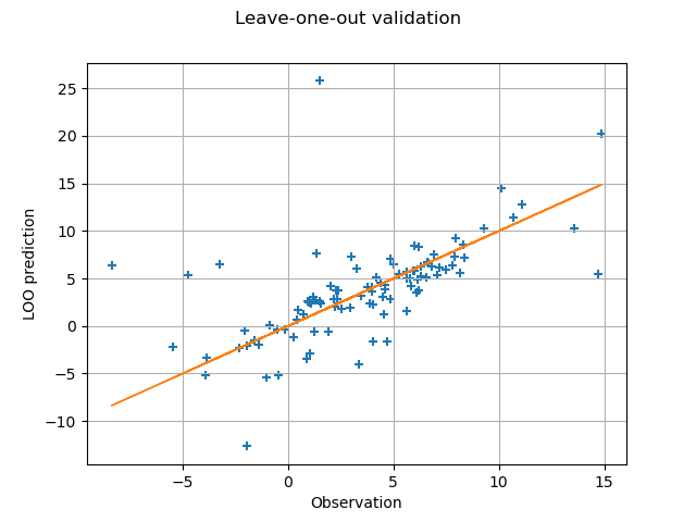
For each point in the training sample, we plot the predicted leave-one-out output prediction depending on the observed output.

graph = ot.Graph("Leave-one-out validation", "Observation", "LOO prediction", True)
cloud = ot.Cloud(yTrain, predictionsLOO)
graph.add(cloud)
curve = ot.Curve(yTrain, yTrain)
graph.add(curve)
view = otv.View(graph)

In the previous method, we must pay attention to the fact that the comparison that we are going to make is not necessarily valid if we use the LARS selection method, because this may lead to a different active basis for each leave-one-out sample.

One limitation of the previous script is that it can be relatively long when the sample size increases or when the size of the functional basis increases. In the next section, we use the analytical formula: this can leads to significant time savings in some cases.

Compute the analytical leave-one-out error¶

Get the diagonal of the projection matrix. This is a Point.

diagonalH = lsqMethod.getHDiag()
print("diagonalH : ", diagonalH.getDimension())

diagonalH :  100

Compute the metamodel predictions.

metamodel = chaosResult.getMetaModel()
yHat = metamodel(xTrain)

Compute the residuals.

residuals = yTrain.asPoint() - yHat.asPoint()

Compute the analytical leave-one-out error: perform elementwise division and exponentiation

delta = np.array(residuals) / (1.0 - np.array(diagonalH))
squaredDelta = delta**2
leaveOneOutMSE = ot.Sample.BuildFromPoint(squaredDelta).computeMean()[0]
print("MSE LOO = ", leaveOneOutMSE)
relativeLOOError = leaveOneOutMSE / yTrain.computeVariance()[0]
q2LeaveOneOut = 1.0 - relativeLOOError
print("Q2 LOO = ", q2LeaveOneOut)

MSE LOO =  27.119388388841855
Q2 LOO =  -0.9306292646908096

We see that the MSE leave-one-out error is equal to the naive LOO error. The numerical differences between the two values are the consequences of the rounding errors in the numerical evaluation of the hat matrix.

otv.View.ShowAll()

OpenTURNS

An Open source initiative for the Treatment of Uncertainties, Risks'N Statistics

Table of Contents

Previous topic

Next topic

This Page