Strong Maximum Test
The Strong Maximum Test is used under the following context: let  be a
probabilistic input
vector with joint density probability
be a
probabilistic input
vector with joint density probability  , let
, let  be the limit state function of
the model and let
be the limit state function of
the model and let  be an event whose probability
 is defined as:
(1)
The probability is evaluated with the FORM and SORM
methods. These methods use the Nataf
isoprobabilistic transformation which maps the
probabilistic model in terms of onto an equivalent model in terms of  independent standard normal random
  (refer to Isoprobabilistic transformations). In that new
 -space,
the event has the new expression defined from the transformed limit state function of the model
-space,
the event has the new expression defined from the transformed limit state function of the model  :
:
 .
.
These analytical methods rely on the assumption that most of the contribution to
comes from points located in the vicinity of a particular point  , the design point, defined in the
-space as the point located on the limit state surface
and of maximal likelihood. Given the probabilistic characteristics of the
-space,
has a geometrical interpretation : it is the point located on the event boundary and at minimal distance
from the center of the -space. Thus, the design point is the result of a constrained
optimization problem.
, the design point, defined in the
-space as the point located on the limit state surface
and of maximal likelihood. Given the probabilistic characteristics of the
-space,
has a geometrical interpretation : it is the point located on the event boundary and at minimal distance
from the center of the -space. Thus, the design point is the result of a constrained
optimization problem.
Both FORM and SORM methods assume that is unique. One important difficulty comes
from the fact that numerical methods involved in the determination of gives no
guaranty of a global optimum: the point to which they converge might be a local optimum only.
In that case, the contribution of the points in the vicinity of the real design point is not
taken into account, and this contribution is the most important one.
Furthermore, even in the case where the global optimum has really been found, there may exist
another local optimum  with
likelihood only slightly inferior to the likelihood of the design point one, which means that it is only slightly
further apart from the
center of the -space than the design point. Thus, points in the vicinity of may
contribute significantly to the probability
and are not taken into account in the FORM and SORM approximations.
with
likelihood only slightly inferior to the likelihood of the design point one, which means that it is only slightly
further apart from the
center of the -space than the design point. Thus, points in the vicinity of may
contribute significantly to the probability
and are not taken into account in the FORM and SORM approximations.
In both cases, the FORM and SORM approximations are of bad quality because they neglect important contributions to
.
The Strong Maximum Test helps to evaluate the quality of the design point resulting from the optimization algorithm. It checks whether the
design point computed is:
the true design point, which means a global maximum point,
a strong design point, which means that there is no other local maximum located on the event boundary and with likelihood only slightly inferior to the likelihood of the design point one.
This verification is very important in order to give sense to the FORM and SORM approximations.
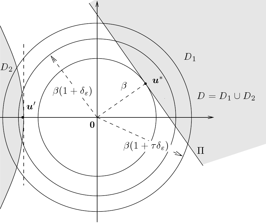
The principle of the Strong Maximum Test relies on the geometrical definition
of the design point.
The objective is to detect all the points in the
ball of radius  which are potentially the real design point (case of
 ) or whose contribution to is not
negligible as regards the approximations Form and SORM (case of
) or whose contribution to is not
negligible as regards the approximations Form and SORM (case of
 ). The contribution of a point is considered as
negligible when its likelihood in the -space is less
than
). The contribution of a point is considered as
negligible when its likelihood in the -space is less
than  times the likelihood of the design point. The
radius
times the likelihood of the design point. The
radius  is the distance to the
-space center upon which points are considered as
negligible .
is the distance to the
-space center upon which points are considered as
negligible .
In order to catch the potential points located on the sphere of radius
(frontier of the zone of prospection), it is
necessary to go a little further : this is why the test samples
the sphere of radius  ,
with
,
with  .
.
Points on the sampled sphere which are in the vicinity of the design
point are less interesting than those verifying the event
and located far from the design point : the latter might reveal
a potential whose contribution to has
to be taken into account. The vicinity of the design point is defined
with the angular parameter  as the cone centered on
and of half-angle .
as the cone centered on
and of half-angle .
The number  of the simulations sampling the sphere of radius
 is determined to ensure that the test detects with a
probability greater than
is determined to ensure that the test detects with a
probability greater than  any point verifying the event
and outside the design point vicinity.
any point verifying the event
and outside the design point vicinity.

The vicinity of the design point is the arc of the sampled sphere which
is inside the half space whose frontier is the linearized limit state
function at the Design Point: the vicinity is
the arc included in the half space  .
.
The Strong Maximum Test proceeds as follows. The User selects the parameters:
the importance level
, where
 ,
,the accuracy level
 , where ,
the confidence level
where  or the
number of points used to sample the sphere. The parameters
are deductible from one other.
or the
number of points used to sample the sphere. The parameters
are deductible from one other.
The Strong Maximum Test will sample the sphere of radius
 , where
 .
.
The test will detect with probability greater than
any point of  whose contribution to is not
negligible (i.e. with density value in the -space
greater than times the density value at the design
point).
whose contribution to is not
negligible (i.e. with density value in the -space
greater than times the density value at the design
point).
The Strong Maximum Test provides:
set 1: all the points detected on the sampled sphere that are in
and outside the design point vicinity, with the
corresponding value of the limit state function,set 2: all the points detected on the sampled sphere that are in
and in the design point vicinity, with the
corresponding value of the limit state function,set 3: all the points detected on the sampled sphere that are outside
and outside the design point vicinity, with the
corresponding value of the limit state function,set 4: all the points detected on the sampled sphere that are outside
but in the vicinity of the design point, with
the corresponding value of the limit state function.
Points are described by their coordinates in the  -space.
The parameter is directly linked to the hypothesis
according to which the boundary of the space is supposed
to be well approximated by a plane near the design point, which is
primordial for a FORM approximation of the probability content of
. Increasing is increasing the area where
the approximation FORM is applied.
The parameter also serves as a measure of distance from
the design point for a hypothetical local maximum:
the larger it is, the further we search for another local maximum.
Numerical experiments show that it is recommended to take
 (see the given reference below).
The following table helps to quantify the parameters of the test for a problem of dimension 5.
|
|
|
|
|
|
|---|---|---|---|---|---|
3.0 |
0.01 |
2.0 |
0.9 |
|
62 |
3.0 |
0.01 |
2.0 |
0.99 |
|
124 |
3.0 |
0.01 |
4.0 |
0.9 |
|
15 |
3.0 |
0.01 |
4.0 |
0.99 |
|
30 |
3.0 |
0.1 |
2.0 |
0.9 |
|
130 |
3.0 |
0.1 |
2.0 |
0.99 |
|
260 |
3.0 |
0.1 |
4.0 |
0.9 |
|
26 |
3.0 |
0.1 |
4.0 |
0.99 |
|
52 |
5.0 |
0.01 |
2.0 |
0.9 |
|
198 |
5.0 |
0.01 |
2.0 |
0.99 |
|
397 |
5.0 |
0.01 |
4.0 |
0.9 |
|
36 |
5.0 |
0.01 |
4.0 |
0.99 |
|
72 |
5.0 |
0.1 |
2.0 |
0.9 |
|
559 |
5.0 |
0.1 |
2.0 |
0.99 |
|
1118 |
5.0 |
0.1 |
4.0 |
0.9 |
|
85 |
5.0 |
0.1 |
4.0 |
0.99 |
|
169 |


|
|
|
|
|
|
|---|---|---|---|---|---|
3.0 |
0.01 |
2.0 |
100 |
|
0.97 |
3.0 |
0.01 |
2.0 |
1000 |
|
1.0 |
3.0 |
0.01 |
4.0 |
100 |
|
1.0 |
3.0 |
0.01 |
4.0 |
1000 |
|
1.0 |
3.0 |
0.1 |
2.0 |
100 |
|
0.83 |
3.0 |
0.1 |
2.0 |
1000 |
|
1.0 |
3.0 |
0.1 |
4.0 |
100 |
|
1.0 |
3.0 |
0.1 |
4.0 |
1000 |
|
1.0 |
5.0 |
0.01 |
2.0 |
100 |
|
0.69 |
5.0 |
0.01 |
2.0 |
1000 |
|
1.0 |
5.0 |
0.01 |
4.0 |
100 |
|
1.0 |
5.0 |
0.01 |
4.0 |
1000 |
|
1.0 |
5.0 |
0.1 |
2.0 |
100 |
|
0.34 |
5.0 |
0.1 |
2.0 |
1000 |
|
0.98 |
5.0 |
0.1 |
4.0 |
100 |
|
0.93 |
5.0 |
0.1 |
4.0 |
1000 |
|
0.99 |
As the Strong Maximum Test involves the computation of values
of the limit state function, which is computationally intensive, it is
interesting to have more than just an indication about the quality of
. In fact, the test gives some information about the
trace of the limit state function on the sphere of radius
centered on the origin of the
-space. Two cases can be distinguished:
- Case 1: set 1 is empty. We are confident on the fact that is a design point verifying the hypothesis
according to which most of the contribution of is
concentrated in the vicinity of . By using the
value of the limit state function on the sample
 , we can check if the limit
state function is reasonably linear in the vicinity of
, which can validate the second hypothesis of
FORM.If the behavior of the limit state function is not linear, we can decide to use an importance sampling version of the Monte Carlo method to compute the probability of failure. However, the information obtained through the Strong Max Test, according to which is the actual design point,
is quite essential : it allows one to construct an effective importance
sampling density, e.g. a multidimensional Gaussian distribution
centered on .
, we can check if the limit
state function is reasonably linear in the vicinity of
, which can validate the second hypothesis of
FORM.If the behavior of the limit state function is not linear, we can decide to use an importance sampling version of the Monte Carlo method to compute the probability of failure. However, the information obtained through the Strong Max Test, according to which is the actual design point,
is quite essential : it allows one to construct an effective importance
sampling density, e.g. a multidimensional Gaussian distribution
centered on . Case 2: set 1 is not empty. There are two possibilities:
We have found some points that suggest that
is
not a strong maximum, because for some points of the sampled
sphere, the value taken by the limit state function is slightly
negative;- We have found some points that suggest that
is not even the global maximum, because for some points of the sampled sphere, the value taken by the limit state function is very negative. In the first case, we can decide to use an importance sampling version of the Monte Carlo method for computing the probability of failure, but with a mixture of e.g. multidimensional gaussian distributions centered on the
 in
(refer to ). In the second case, we can restart the search of
the design point by starting at the detected .
in
(refer to ). In the second case, we can restart the search of
the design point by starting at the detected .
- We have found some points that suggest that