LinearLeastSquares
- class LinearLeastSquares(*args)
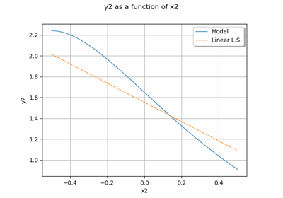
First order polynomial response surface by least squares.
- Parameters:
- dataIn2-d sequence of float
Input data.
- dataOut2-d sequence of float
Output data. If not specified, this sample is computed such as:
 .
.
Methods
Accessor to the object's name.
Get the constant vector of the approximation.
Get the input data.
Get the output data.
Get the linear matrix of the approximation.
Get an approximation of the function.
getName()Accessor to the object's name.
hasName()Test if the object is named.
run()Perform the least squares approximation.
setDataOut(dataOut)Set the output data.
setName(name)Accessor to the object's name.
See also
Notes
Instead of replacing the model response
 for a local
approximation around a given set
for a local
approximation around a given set  of input parameters as in
Taylor approximations, one may seek a global approximation of
over its whole domain of definition. A common choice to
this end is global polynomial approximation.
of input parameters as in
Taylor approximations, one may seek a global approximation of
over its whole domain of definition. A common choice to
this end is global polynomial approximation.We consider here a global approximation of the model response using a linear function:

where
 is a set of unknown coefficients
and the family
is a set of unknown coefficients
and the family  gathers the constant monomial
 and the monomials of degree one
  . Using the vector
notation
. Using the vector
notation  and
and
 ,
this rewrites:
,
this rewrites:
A global approximation of the model response over its whole definition domain is sought. To this end, the coefficients
 may be computed using a
least squares regression approach. In this context, an experimental design
may be computed using a
least squares regression approach. In this context, an experimental design
 , i.e. a set of realizations of
input parameters is required, as well as the corresponding model evaluations
, i.e. a set of realizations of
input parameters is required, as well as the corresponding model evaluations
 .
.The following minimization problem has to be solved:

The solution is given by:

where:

Examples
>>> import openturns as ot
>>> formulas = ['cos(x1 + x2)', '(x2 + 1) * exp(x1 - 2 * x2)']
>>> f = ot.SymbolicFunction(['x1', 'x2'], formulas)
>>> X  = [[0.5,0.5], [-0.5,-0.5], [-0.5,0.5], [0.5,-0.5]]
>>> X += [[0.25,0.25], [-0.25,-0.25], [-0.25,0.25], [0.25,-0.25]]
>>> Y = f(X)
>>> myLeastSquares = ot.LinearLeastSquares(X, Y)
>>> myLeastSquares.run()
>>> mm = myLeastSquares.getMetaModel()
>>> x = [0.1, 0.1]
>>> y = mm(x)
- __init__(*args)
- getClassName()
Accessor to the object’s name.
- Returns:
- class_namestr
The object class name (object.__class__.__name__).
- getConstant()
Get the constant vector of the approximation.
- Returns:
- constantVector
Point Constant vector of the approximation, equal to
 .
.
- constantVector
- getDataOut()
Get the output data.
- Returns:
- dataOut
Sample Output data. If not specified in the constructor, the sample is computed such as:
.
- dataOut
- getLinear()
Get the linear matrix of the approximation.
- Returns:
- linearMatrix
Matrix Linear matrix of the approximation of the function
 .
.
- linearMatrix
- getMetaModel()
Get an approximation of the function.
- Returns:
- approximation
Function An approximation of the function
by Linear Least Squares.
- approximation
- getName()
Accessor to the object’s name.
- Returns:
- namestr
The name of the object.
- hasName()
Test if the object is named.
- Returns:
- hasNamebool
True if the name is not empty.
- run()
Perform the least squares approximation.
- setDataOut(dataOut)
Set the output data.
- Parameters:
- dataOut2-d sequence of float
Output data.
- setName(name)
Accessor to the object’s name.
- Parameters:
- namestr
The name of the object.