Using otagrum

import openturns as ot
import pyAgrum as gum
from matplotlib import pylab as plt
import otagrum

def showDot(dotstring):
    try:
        # fails outside notebook
        import pyAgrum.lib.notebook as gnb

        gnb.showDot(dotstring)
    except ImportError:
        import pydot
        from io import BytesIO

        graph = pydot.graph_from_dot_data(dotstring)[0]
        with BytesIO() as f:
            f.write(graph.create_png())
            f.seek(0)
            img = plt.imread(f)
        fig = plt.imshow(img)
        fig.axes.axis("off")
        plt.show()

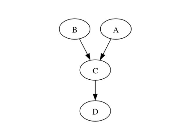
Creating the CBN structure We begin by creating the CBN that will be used throughout this example.

To do so, we need a NamedDAG structure…

dag = gum.DAG()

mapping = {}
mapping["A"] = dag.addNode()  # Add node A
mapping["B"] = dag.addNode()  # Add node B
mapping["C"] = dag.addNode()  # Add node C
mapping["D"] = dag.addNode()  # Add node D

dag.addArc(mapping["A"], mapping["C"])  # Arc A -> C
dag.addArc(mapping["B"], mapping["C"])  # Arc B -> C
dag.addArc(mapping["C"], mapping["D"])  # Arc C -> D

dag

(pyAgrum.DAG@0x55e6a8bd0d30) {0,1,2,3} , {2->3,0->2,1->2}

structure = otagrum.NamedDAG(dag, list(mapping.keys()))

showDot(structure.toDot())

<IPython.core.display.SVG object>

Parameters of the CBN … and a collection of marginals and local conditional copulas.

m_list = [ot.Uniform(0.0, 1.0) for i in range(structure.getSize())]  # Local marginals
lcc_list = []  # Local Conditional Copulas
for i in range(structure.getSize()):
    dim_lcc = structure.getParents(i).getSize() + 1
    R = ot.CorrelationMatrix(dim_lcc)
    for j in range(dim_lcc):
        for k in range(j):
            R[j, k] = 0.6
    lcc_list.append(ot.Normal([0.0] * dim_lcc, [1.0] * dim_lcc, R).getCopula())

Now that we have a NamedDAG structure and a collection of local conditional copulas, we can construct a CBN.

cbn = otagrum.ContinuousBayesianNetwork(structure, m_list, lcc_list)

Having a CBN, we can now sample from it.

ot.RandomGenerator.SetSeed(10)  # Set random seed
sample = cbn.getSample(1000)
train = sample[:-100]
test = sample[-100:]

Learning the structure with continuous PC: Now that we have data, we can use it to learn the structure with the continuous PC algorithm.

learner = otagrum.ContinuousPC(sample, 5, 0.1)

We first learn the skeleton, that is the undirected structure.

skeleton = learner.learnSkeleton()

skeleton

(pyAgrum.UndiGraph@0x55e6a7ea6c00) {0,1,2,3} , {2--3,0--2,1--2}

Then we look for the v-structures, leading to a Partially Directed Acyclic Graph (PDAG)

pdag = learner.learnPDAG()

pdag

(pyAgrum.MixedGraph@0x55e6a8d13680) {0,1,2,3} , {1->2,0->2} , {2--3}

Finally, the remaining edges are oriented by propagating constraints

ndag = learner.learnDAG()

showDot(ndag.toDot())

<IPython.core.display.SVG object>

The true structure has been recovered. Learning with continuous MIIC Otagrum provides another learning algorithm to learn the structure: the continuous MIIC algorithm.

learner = otagrum.ContinuousMIIC(sample)

This algorithm relies on the computing of mutual information which is done through the copula function. Hence, a copula model for the data is needed. The continuous MIIC algorithm can make use of Gaussian copulas (parametric) or Bernstein copulas (non-parametric) to compute mutual information. Moreover, due to finite sampling size, the mutual information estimators need to be corrected. Two kind of correction are provided: NoCorr (no correction) or Naive (a fixed correction is subtracted from the raw mutual information estimators). Those behaviours can be changed as follows:

learner.setCMode(otagrum.CorrectedMutualInformation.CModeTypes_Bernstein) # By default

learner.setCMode(
    otagrum.CorrectedMutualInformation.CModeTypes_Gaussian
)  # To use Gaussian copulas
learner.setKMode(otagrum.CorrectedMutualInformation.KModeTypes_Naive)  # By default
# learner.setKMode(otagrum.CorrectedMutualInformation.KModeTypes_NoCorr) # To use the raw estimators
learner.setAlpha(
    0.01
)  # Set the correction value for the Naive behaviour, it is set to 0.01 by default

As with PC algorithm we can learn the skeleton, PDAG and DAG using

skeleton = learner.learnSkeleton()

skeleton

(pyAgrum.UndiGraph@0x55e6a8d23d00) {0,1,2,3} , {2--3,0--2,1--2}

pdag = learner.learnPDAG()

pdag

(pyAgrum.MixedGraph@0x55e6a8cadb10) {0,1,2,3} , {2->3,1->2,0->2} , {}

dag = learner.learnDAG()

showDot(dag.toDot())

<IPython.core.display.SVG object>

Learning parameters Bernstein copulas are used to learn the local conditional copulas associated to each node

m_list = []
lcc_list = []
for i in range(train.getDimension()):
    m_list.append(ot.UniformFactory().build(train.getMarginal(i)))
    indices = [i] + [int(n) for n in ndag.getParents(i)]
    dim_lcc = len(indices)
    if dim_lcc == 1:
        bernsteinCopula = ot.IndependentCopula(1)
    elif dim_lcc > 1:
        K = otagrum.ContinuousTTest.GetK(len(train), dim_lcc)
        bernsteinCopula = ot.EmpiricalBernsteinCopula(
            train.getMarginal(indices), K, False
        )
    lcc_list.append(bernsteinCopula)

We can now create the learned CBN

lcbn = otagrum.ContinuousBayesianNetwork(ndag, m_list, lcc_list)  # Learned CBN

And compare the mean loglikelihood between the true and the learned models

def compute_mean_LL(cbn, test):
    ll = 0
    for t in test:
        ll += cbn.computeLogPDF(t)
    ll /= len(test)
    return ll

true_LL = compute_mean_LL(cbn, test)
print(true_LL)

0.31620906143480526

exp_LL = compute_mean_LL(lcbn, test)
print(exp_LL)

0.15241697100666607