POD Summary
[1]:
# import relevant module
import openturns as ot
import otpod
# enable display figure in notebook
try:
    %matplotlib inline
except:
    pass
/calcul/home/dumas/anaconda/lib/python3.6/site-packages/sklearn/ensemble/weight_boosting.py:29: DeprecationWarning: numpy.core.umath_tests is an internal NumPy module and should not be imported. It will be removed in a future NumPy release.
  from numpy.core.umath_tests import inner1d
Generate data
[2]:
inputSample = ot.Sample(
    [[4.59626812e+00, 7.46143339e-02, 1.02231538e+00, 8.60042277e+01],
    [4.14315790e+00, 4.20801346e-02, 1.05874908e+00, 2.65757364e+01],
    [4.76735111e+00, 3.72414824e-02, 1.05730385e+00, 5.76058433e+01],
    [4.82811977e+00, 2.49997658e-02, 1.06954641e+00, 2.54461380e+01],
    [4.48961094e+00, 3.74562922e-02, 1.04943946e+00, 6.19483646e+00],
    [5.05605334e+00, 4.87599783e-02, 1.06520409e+00, 3.39024904e+00],
    [5.69679328e+00, 7.74915877e-02, 1.04099514e+00, 6.50990466e+01],
    [5.10193991e+00, 4.35520544e-02, 1.02502536e+00, 5.51492592e+01],
    [4.04791970e+00, 2.38565932e-02, 1.01906882e+00, 2.07875350e+01],
    [4.66238956e+00, 5.49901237e-02, 1.02427200e+00, 1.45661275e+01],
    [4.86634219e+00, 6.04693570e-02, 1.08199374e+00, 1.05104730e+00],
    [4.13519347e+00, 4.45225831e-02, 1.01900124e+00, 5.10117047e+01],
    [4.92541940e+00, 7.87692335e-02, 9.91868726e-01, 8.32302238e+01],
    [4.70722074e+00, 6.51799251e-02, 1.10608515e+00, 3.30181002e+01],
    [4.29040932e+00, 1.75426222e-02, 9.75678838e-01, 2.28186756e+01],
    [4.89291400e+00, 2.34997929e-02, 1.07669835e+00, 5.38926138e+01],
    [4.44653744e+00, 7.63175936e-02, 1.06979154e+00, 5.19109415e+01],
    [3.99977452e+00, 5.80430585e-02, 1.01850716e+00, 7.61988190e+01],
    [3.95491570e+00, 1.09302814e-02, 1.03687664e+00, 6.09981789e+01],
    [5.16424368e+00, 2.69026464e-02, 1.06673711e+00, 2.88708887e+01],
    [5.30491620e+00, 4.53802273e-02, 1.06254792e+00, 3.03856837e+01],
    [4.92809155e+00, 1.20616369e-02, 1.00700410e+00, 7.02512744e+00],
    [4.68373805e+00, 6.26028935e-02, 1.05152117e+00, 4.81271603e+01],
    [5.32381954e+00, 4.33013582e-02, 9.90522007e-01, 6.56015973e+01],
    [4.35455857e+00, 1.23814619e-02, 1.01810539e+00, 1.10769534e+01]])

signals = ot.Sample(
    [[ 37.305445], [ 35.466919], [ 43.187991], [ 45.305165], [ 40.121222], [ 44.609524],
     [ 45.14552 ], [ 44.80595 ], [ 35.414039], [ 39.851778], [ 42.046049], [ 34.73469 ],
     [ 39.339349], [ 40.384559], [ 38.718623], [ 46.189709], [ 36.155737], [ 31.768369],
     [ 35.384313], [ 47.914584], [ 46.758537], [ 46.564428], [ 39.698493], [ 45.636588],
     [ 40.643948]])
Compute POD with several methods
The object POD summary enables the user to compute the POD with all available techniques. techniques can be activated or not thanks to the method setMethodActive. Then results can be printed or saved in a file to be compared. Moreover all graphs from the studies can be saved in a given directory.
The techniques are all activated by default :
Univariate linear model with Gaussian residuals,
Univariate linear model with no hypothesis on the residuals (Binomial),
Univariate linear model with kernel smoothing on the residuals,
Quantile regression,
Polynomial chaos,
Kriging (if input dimension > 1)
[3]:
# signal detection threshold
detection = 38.
# The POD summary take
POD = otpod.PODSummary(inputSample, signals, detection, 25)
# The main parameters can modified :
# The number of simulation to compute the confidence level
POD.setSimulationSize(50)
# The number of Monte Carlo simulation to compute the POD for polynomial chaos and kriging
POD.setSamplingSize(200)
# Deactivate the quantile regression technique
POD.setMethodActive('QuantileRegression', False)
# Finally run
POD.run()
Start univariate linear model analysis...

Start univariate linear model POD with Gaussian residuals...

Start univariate linear model POD with no hypothesis on the residuals...

Start univariate linear model POD with kernel smoothing on the residuals...
Computing POD (bootstrap): [==================================================] 100.00% Done
INFO:root:Censored data are not taken into account : the polynomial chaos model is only built on filtered data.
Start polynomial chaos POD...
Start build polynomial chaos model...
Polynomial chaos model completed
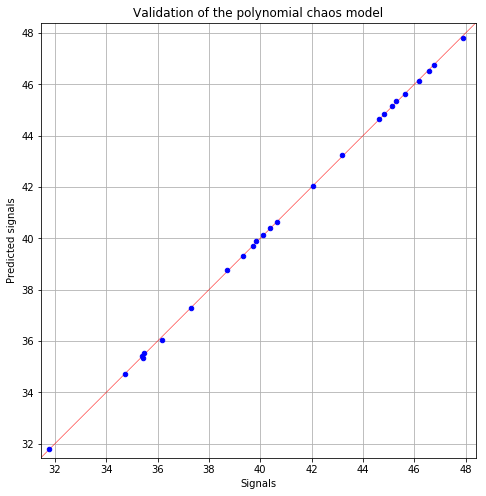
Polynomial chaos validation R2 (>0.8) : 0.9999
Polynomial chaos validation Q2 (>0.8) : 0.9987
Computing POD per defect: [==================================================] 100.00% Done
INFO:root:Censored data are not taken into account : the kriging model is only built on filtered data.
Start kriging POD...
Start optimizing covariance model parameters...
Kriging optimizer completed
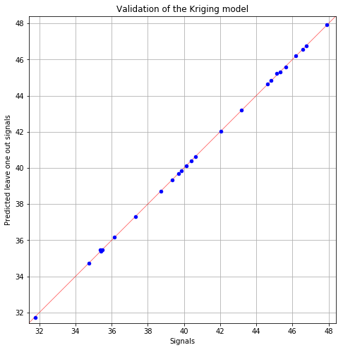
kriging validation Q2 (>0.9): 1.0000
Computing POD per defect: [==================================================] 100.00% Done
Access to the dictionnary of the active methods
[4]:
POD.getMethodActive()
[4]:
{'LinearGauss': True,
 'LinearBinomial': True,
 'LinearKernelSmoothing': True,
 'QuantileRegression': False,
 'PolynomialChaos': True,
 'Kriging': True}
Show results
It is shown the linear analysis results as well as the validation results of each model with the detection size computed for a given probability level and confidence level. These both values can be changed as parameters of the printResults method. The default values are probability level = 0.9 and confidence level = 0.95.
A warning is printed when the detection size with a technique returns an error. In this case, the return value is -1.
[5]:
print(POD.getResults())
INFO:root:Warning : For polynomial chaos, kriging, results are given for filtered data.
--------------------------------------------------------------------------------
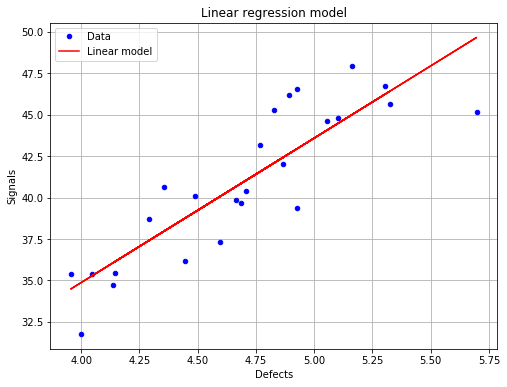
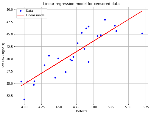
Linear model analysis results
--------------------------------------------------------------------------------
Box Cox parameter : Not enabled
Uncensored Censored
Intercept coefficient : 0.02 0.02
Slope coefficient : 8.71 8.71
Standard error of the estimate : 2.29 2.2
Confidence interval on coefficients
Intercept coefficient : [-10.03, 10.07]
Slope coefficient : [6.58, 10.85]
Level : 0.95
Quality of regression
R2 (> 0.8): 0.76 0.76
--------------------------------------------------------------------------------
--------------------------------------------------------------------------------
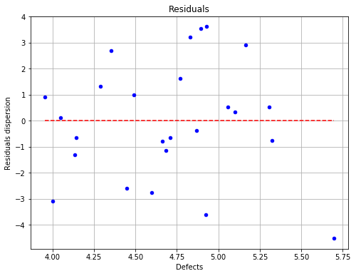
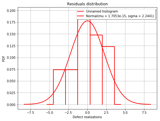
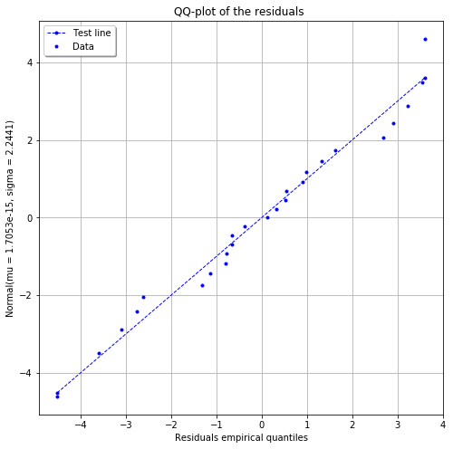
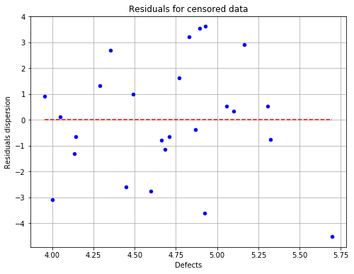
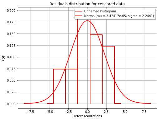
Residuals analysis results
--------------------------------------------------------------------------------
Fitted distribution (uncensored) : Normal(mu = 1.7053e-15, sigma = 2.2441)
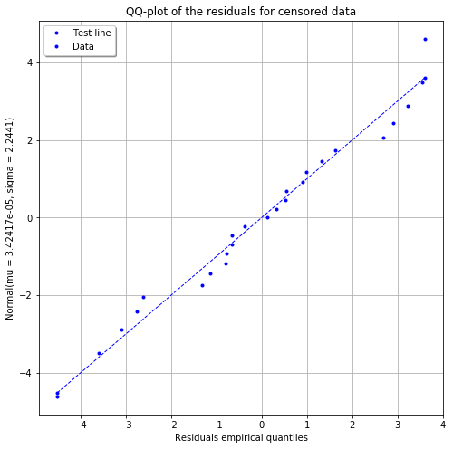
Fitted distribution (censored) : Normal(mu = 3.42417e-05, sigma = 2.2441)
Uncensored Censored
Distribution fitting test
Kolmogorov p-value (> 0.05): 0.99 0.99
Normality test
Anderson Darling p-value (> 0.05): 0.76 0.76
Cramer Von Mises p-value (> 0.05): 0.83 0.83
Zero residual mean test
p-value (> 0.05): 1.0 1.0
Homoskedasticity test (constant variance)
Breush Pagan p-value (> 0.05): 0.09 0.09
Harrison McCabe p-value (> 0.05): 0.21 0.23
Non autocorrelation test
Durbin Watson p-value (> 0.05): 0.34 0.34
--------------------------------------------------------------------------------
--------------------------------------------------------------------------------
Model validation results
--------------------------------------------------------------------------------
Uncensored Censored
R2 Q2 R2
Linear Regression (> 0.8): 0.76 0.76
Polynomial Chaos (> 0.8): 1.0 1.0
Kriging (> 0.8): 1.0
--------------------------------------------------------------------------------
--------------------------------------------------------------------------------
POD results
--------------------------------------------------------------------------------
a90 a90/95
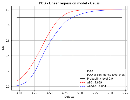
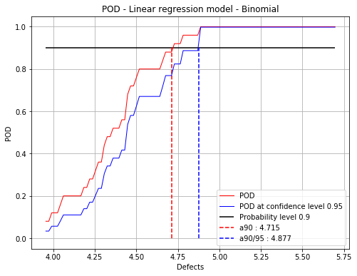
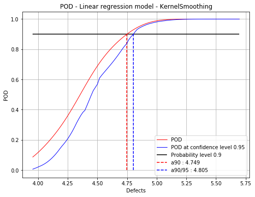
Linear Regression
Gaussian residuals : 4.69 4.88
No residuals hypothesis : 4.71 4.88
Kernel smoothing on residuals : 4.75 4.81
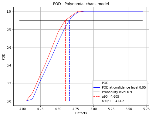
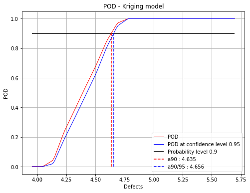
Polynomial chaos : 4.6 4.66
Kriging : 4.63 4.66
--------------------------------------------------------------------------------
Warning : For polynomial chaos, kriging, results are given for filtered data.
Results can be displayed for another probability and confidence level.
[6]:
print(POD.getResults(0.8, 0.9))
INFO:root:Warning : For polynomial chaos, kriging, results are given for filtered data.
--------------------------------------------------------------------------------
         Linear model analysis results
--------------------------------------------------------------------------------
Box Cox parameter :                               Not enabled

                                                   Uncensored      Censored

Intercept coefficient :                                  0.02          0.02
Slope coefficient :                                      8.71          8.71
Standard error of the estimate :                         2.29           2.2

Confidence interval on coefficients
Intercept coefficient :                         [-10.03, 10.07]
Slope coefficient :                             [6.58, 10.85]
Level :                                                  0.95

Quality of regression
R2 (> 0.8):                                              0.76          0.76
--------------------------------------------------------------------------------

--------------------------------------------------------------------------------
         Residuals analysis results
--------------------------------------------------------------------------------
Fitted distribution (uncensored) :              Normal(mu = 1.7053e-15, sigma = 2.2441)
Fitted distribution (censored) :                Normal(mu = 3.42417e-05, sigma = 2.2441)

                                                   Uncensored      Censored
Distribution fitting test
Kolmogorov p-value (> 0.05):                             0.99          0.99

Normality test
Anderson Darling p-value (> 0.05):                       0.76          0.76
Cramer Von Mises p-value (> 0.05):                       0.83          0.83

Zero residual mean test
p-value (> 0.05):                                         1.0           1.0

Homoskedasticity test (constant variance)
Breush Pagan p-value (> 0.05):                           0.09          0.09
Harrison McCabe p-value (> 0.05):                        0.21          0.23

Non autocorrelation test
Durbin Watson p-value (> 0.05):                          0.34          0.34
--------------------------------------------------------------------------------


--------------------------------------------------------------------------------
         Model validation results
--------------------------------------------------------------------------------
                                                      Uncensored   Censored

                                                   R2         Q2         R2

Linear Regression (> 0.8):                       0.76                  0.76
Polynomial Chaos (> 0.8):                         1.0        1.0
Kriging (> 0.8):                                             1.0
--------------------------------------------------------------------------------

--------------------------------------------------------------------------------
         POD results
--------------------------------------------------------------------------------
                                                          a80        a80/90
Linear Regression
Gaussian residuals :                                     4.58          4.67
No residuals hypothesis :                                4.64          4.68
Kernel smoothing on residuals :                          4.61          4.68

Polynomial chaos :                                       4.52          4.58
Kriging :                                                4.57          4.59
--------------------------------------------------------------------------------

Warning : For polynomial chaos, kriging, results are given for filtered data.
Save results
The results can be saved in a text or csv file. As for the print method, the probability level and confidence level can be specified as parameters.
[7]:
POD.saveResults('results.csv', probabilityLevel=0.9, confidenceLevel=0.95)
Draw and save graphs
All available graphs can be saved using the method saveGraphs. A specific directory and the extension of the files can be given as parameters. As before the probability level and confidence level can also be chosen by the user.
The warning is also printed here for the polynomial chaos because the detection size at the given probability level cannot be computed. A solution is to set probabilityLevel = None.
[8]:
# return a list a figure
fig = POD.drawGraphs('./figure/', 'png', probabilityLevel=0.9, confidenceLevel=0.95)

for i in range(len(fig)):
    fig[i].show()
/calcul/home/dumas/anaconda/lib/python3.6/site-packages/matplotlib/figure.py:459: UserWarning: matplotlib is currently using a non-GUI backend, so cannot show the figure
  "matplotlib is currently using a non-GUI backend, "
[ ]: