Calibration of the Chaboche mecanical model¶

Deterministic model¶

The Chaboche mecanical law predicts the stress depending on the strain:

$\sigma = G(\epsilon,R,C,\gamma) = R + \frac{C}{\gamma} (1-\exp(-\gamma\epsilon))$

where:

$\epsilon$ is the strain,
$\sigma$ is the stress (Pa),
$R$ , $C$ , $\gamma$ are the parameters.

The variables have the following distributions and are supposed to be independent.

Random var.	Distribution
$R$	Lognormal ( $\mu = 750$ MPa, $\sigma = 11$ MPa)
$C$	Normal ( $\mu = 2750$ MPa, $\sigma = 250$ MPa)
$\gamma$	Normal ( $\mu = 10$ , $\sigma = 2$ )
$\epsilon$	Uniform(a=0, b=0.07).

Parameters to calibrate¶

The vector of parameters to calibrate is:

$\theta = (R,C,\gamma).$

We set:

$R = 750\times 10^6$ ,
$C = 2750\times 10^6$ ,
$\gamma = 10$ .

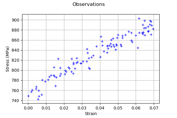
Observations¶

In order to create a calibration problem, we make the hypothesis that the strain has the following distribution:

$\epsilon \sim Uniform(0,0.07).$

Moreover, we consider a gaussian noise on the observed constraint:

$\epsilon_\sigma \sim \mathcal{N} \left(0,10\times 10^6\right)$

and we make the hypothesis that the observation errors are independent. We set the number of observations to:

$n = 100.$

We generate a Monte-Carlo samplg with size $n$ :

$\sigma_i = G(\epsilon_i,R,C,\gamma) + (\epsilon_\sigma)_i,$

for $i = 1,..., n$ . The observations are the pairs $\{(\epsilon_i,\sigma_i)\}_{i=1,...,n}$ , i.e. each observation is a couple made of the strain and the corresponding stress.

Thanks to¶

Antoine Dumas, Phimeca

References¶

1. Lemaitre and J. L. Chaboche (2002) “Mechanics of solid materials” Cambridge University Press.

Generate the observations¶

[1]:

import numpy as np
import openturns as ot

Define the model.

[2]:

def modelChaboche(X):
    strain, R, C, gamma = X
    stress = R + C * (1 - np.exp(-gamma * strain)) / gamma
    return [stress]

Create the Python function.

[3]:

g = ot.PythonFunction(4, 1, modelChaboche)

Define the random vector.

[4]:

Strain = ot.Uniform(0,0.07)
unknownR = 750e6
unknownC = 2750e6
unknownGamma = 10
R = ot.Dirac(unknownR)
C = ot.Dirac(unknownC)
Gamma = ot.Dirac(unknownGamma)

Strain.setDescription(["Strain"])
R.setDescription(["R"])
C.setDescription(["C"])
Gamma.setDescription(["Gamma"])

Create the joint input distribution function.

[5]:

inputDistribution = ot.ComposedDistribution([Strain, R, C, Gamma])

Create the Monte-Carlo sample.

[6]:

sampleSize = 100
inputSample = inputDistribution.getSample(sampleSize)
outputStress = g(inputSample)
outputStress[0:5]

[6]:

	y0
0	848051716.1855512
1	876763726.8422453
2	774845768.8873012
3	756186139.4613488
4	809312377.4983335

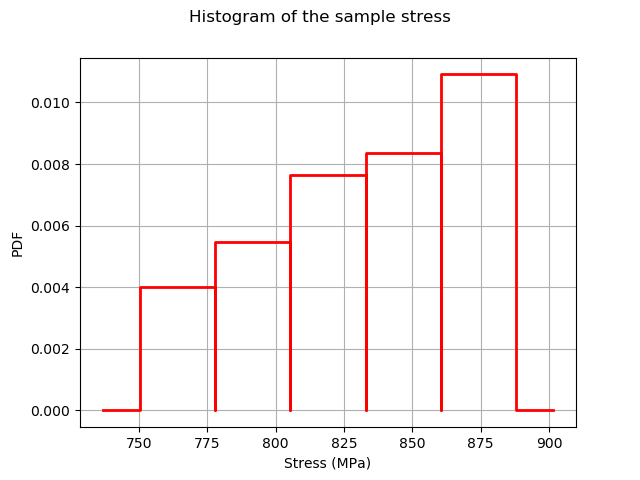
Plot the histogram of the output.

[7]:

histoGraph = ot.HistogramFactory().build(outputStress/1.e6).drawPDF()
histoGraph.setTitle("Histogram of the sample stress")
histoGraph.setXTitle("Stress (MPa)")
histoGraph.setLegends([""])
histoGraph

[7]:

../../_images/examples_calibration_calibration_chaboche_14_0.png

Generate observation noise.

[8]:

stressObservationNoiseSigma = 10.e6 # (Pa)
noiseSigma = ot.Normal(0.,stressObservationNoiseSigma)
sampleNoiseH = noiseSigma.getSample(sampleSize)
observedStress = outputStress + sampleNoiseH

[9]:

observedStrain = inputSample[:,0]

[10]:

graph = ot.Graph("Observations","Strain","Stress (MPa)",True)
cloud = ot.Cloud(observedStrain,observedStress/1.e6)
graph.add(cloud)
graph

[10]:

../../_images/examples_calibration_calibration_chaboche_18_0.png

A calibration analysis class¶

[11]:

"""
A graphics class to analyze the results of calibration.
"""

import pylab as pl
import openturns as ot
import openturns.viewer as otv

class CalibrationAnalysis:
    def __init__(self,calibrationResult,model,inputObservations,outputObservations):
        """
        Plots the prior and posterior distribution of the calibrated parameter theta.

        Parameters
        ----------
        calibrationResult : :class:`~openturns.calibrationResult`
            The result of a calibration.

        model : 2-d sequence of float
            The function to calibrate.

        inputObservations : :class:`~openturns.Sample`
            The sample of input values of the model linked to the observations.

        outputObservations : 2-d sequence of float
            The sample of output values of the model linked to the observations.
        """
        self.model = model
        self.outputAtPrior = None
        self.outputAtPosterior = None
        self.calibrationResult = calibrationResult
        self.observationColor = "blue"
        self.priorColor = "red"
        self.posteriorColor = "green"
        self.inputObservations = inputObservations
        self.outputObservations = outputObservations
        self.unitlength = 6 # inch
        # Compute yAtPrior
        meanPrior = calibrationResult.getParameterPrior().getMean()
        model.setParameter(meanPrior)
        self.outputAtPrior=model(inputObservations)
        # Compute yAtPosterior
        meanPosterior = calibrationResult.getParameterPosterior().getMean()
        model.setParameter(meanPosterior)
        self.outputAtPosterior=model(inputObservations)
        return None

    def drawParameterDistributions(self):
        """
        Plots the prior and posterior distribution of the calibrated parameter theta.
        """
        thetaPrior = self.calibrationResult.getParameterPrior()
        thetaDescription = thetaPrior.getDescription()
        thetaPosterior = self.calibrationResult.getParameterPosterior()
        thetaDim = thetaPosterior.getDimension()
        fig = pl.figure(figsize=(12, 4))
        for i in range(thetaDim):
            graph = ot.Graph("",thetaDescription[i],"PDF",True,"topright")
            # Prior distribution
            thetaPrior_i = thetaPrior.getMarginal(i)
            priorPDF = thetaPrior_i.drawPDF()
            priorPDF.setColors([self.priorColor])
            priorPDF.setLegends(["Prior"])
            graph.add(priorPDF)
            # Posterior distribution
            thetaPosterior_i = thetaPosterior.getMarginal(i)
            postPDF = thetaPosterior_i.drawPDF()
            postPDF.setColors([self.posteriorColor])
            postPDF.setLegends(["Posterior"])
            graph.add(postPDF)
            '''
            If the prior is a Dirac, set the vertical axis bounds to the posterior.
            Otherwise, the Dirac set to [0,1], where the 1 can be much larger
            than the maximum PDF of the posterior.
            '''
            if (thetaPrior_i.getName()=="Dirac"):
                # The vertical (PDF) bounds of the posterior
                postbb = postPDF.getBoundingBox()
                pdf_upper = postbb.getUpperBound()[1]
                pdf_lower = postbb.getLowerBound()[1]
                # Set these bounds to the graph
                bb = graph.getBoundingBox()
                graph_upper = bb.getUpperBound()
                graph_upper[1] = pdf_upper
                bb.setUpperBound(graph_upper)
                graph_lower = bb.getLowerBound()
                graph_lower[1] = pdf_lower
                bb.setLowerBound(graph_lower)
                graph.setBoundingBox(bb)
            # Add it to the graphics
            ax = fig.add_subplot(1, thetaDim, i+1)
            _ = otv.View(graph, figure=fig, axes=[ax])
        return fig

    def drawObservationsVsPredictions(self):
        """
        Plots the output of the model depending
        on the output observations before and after calibration.
        """

        ySize = self.outputObservations.getSize()
        yDim = self.outputObservations.getDimension()
        graph = ot.Graph("","Observations","Predictions",True,"topleft")
        # Plot the diagonal
        if (yDim==1):
            graph = self._drawObservationsVsPredictions1Dimension(self.outputObservations,self.outputAtPrior,self.outputAtPosterior)
        elif (ySize==1):
            outputObservations = ot.Sample(self.outputObservations[0],1)
            outputAtPrior = ot.Sample(self.outputAtPrior[0],1)
            outputAtPosterior = ot.Sample(self.outputAtPosterior[0],1)
            graph = self._drawObservationsVsPredictions1Dimension(outputObservations,outputAtPrior,outputAtPosterior)
        else:
            fig = pl.figure(figsize=(self.unitlength*yDim, self.unitlength))
            for i in range(yDim):
                outputObservations = self.outputObservations[:,i]
                outputAtPrior = self.outputAtPrior[:,i]
                outputAtPosterior = self.outputAtPosterior[:,i]
                graph = self._drawObservationsVsPredictions1Dimension(outputObservations,outputAtPrior,outputAtPosterior)
                ax = fig.add_subplot(1, yDim, i+1)
                _ = otv.View(graph, figure=fig, axes=[ax])

        return graph

    def _drawObservationsVsPredictions1Dimension(self,outputObservations,outputAtPrior,outputAtPosterior):
        """
        Plots the output of the model depending
        on the output observations before and after calibration.
        Can manage only 1D samples.
        """
        yDim = outputObservations.getDimension()
        ydescription = outputObservations.getDescription()
        xlabel = "%s Observations" % (ydescription[0])
        ylabel = "%s Predictions" % (ydescription[0])
        graph = ot.Graph("",xlabel,ylabel,True,"topleft")
        # Plot the diagonal
        if (yDim==1):
            curve = ot.Curve(outputObservations, outputObservations)
            curve.setColor(self.observationColor)
            graph.add(curve)
        else:
            raise TypeError('Output observations are not 1D.')
        # Plot the predictions before
        yPriorDim = outputAtPrior.getDimension()
        if (yPriorDim==1):
            cloud = ot.Cloud(outputObservations, outputAtPrior)
            cloud.setColor(self.priorColor)
            cloud.setLegend("Prior")
            graph.add(cloud)
        else:
            raise TypeError('Output prior predictions are not 1D.')
        # Plot the predictions after
        yPosteriorDim = outputAtPosterior.getDimension()
        if (yPosteriorDim==1):
            cloud = ot.Cloud(outputObservations, outputAtPosterior)
            cloud.setColor(self.posteriorColor)
            cloud.setLegend("Posterior")
            graph.add(cloud)
        else:
            raise TypeError('Output posterior predictions are not 1D.')
        return graph

    def drawResiduals(self):
        """
        Plot the distribution of the residuals and
        the distribution of the observation errors.
        """
        ySize = self.outputObservations.getSize()
        yDim = self.outputObservations.getDimension()
        yPriorSize = self.outputAtPrior.getSize()
        yPriorDim = self.outputAtPrior.getDimension()
        if (yDim==1):
            observationsError = self.calibrationResult.getObservationsError()
            graph = self._drawResiduals1Dimension(self.outputObservations,self.outputAtPrior,self.outputAtPosterior,observationsError)
        elif (ySize==1):
            outputObservations = ot.Sample(self.outputObservations[0],1)
            outputAtPrior = ot.Sample(self.outputAtPrior[0],1)
            outputAtPosterior = ot.Sample(self.outputAtPosterior[0],1)
            observationsError = self.calibrationResult.getObservationsError()
            # In this case, we cannot draw observationsError ; just
            # pass the required input argument, but it is not actually used.
            graph = self._drawResiduals1Dimension(outputObservations,outputAtPrior,outputAtPosterior,observationsError)
        else:
            observationsError = self.calibrationResult.getObservationsError()
            fig = pl.figure(figsize=(self.unitlength*yDim, self.unitlength))
            for i in range(yDim):
                outputObservations = self.outputObservations[:,i]
                outputAtPrior = self.outputAtPrior[:,i]
                outputAtPosterior = self.outputAtPosterior[:,i]
                observationsErrorYi = observationsError.getMarginal(i)
                graph = self._drawResiduals1Dimension(outputObservations,outputAtPrior,outputAtPosterior,observationsErrorYi)
                ax = fig.add_subplot(1, yDim, i+1)
                _ = otv.View(graph, figure=fig, axes=[ax])
        return graph

    def _drawResiduals1Dimension(self,outputObservations,outputAtPrior,outputAtPosterior,observationsError):
        """
        Plot the distribution of the residuals and
        the distribution of the observation errors.
        Can manage only 1D samples.
        """
        ydescription = outputObservations.getDescription()
        xlabel = "%s Residuals" % (ydescription[0])
        graph = ot.Graph("Residuals analysis",xlabel,"Probability distribution function",True,"topright")
        yDim = outputObservations.getDimension()
        yPriorDim = outputAtPrior.getDimension()
        yPosteriorDim = outputAtPrior.getDimension()
        if (yDim==1) and (yPriorDim==1) :
            posteriorResiduals = outputObservations - outputAtPrior
            kernel = ot.KernelSmoothing()
            fittedDist = kernel.build(posteriorResiduals)
            residualPDF = fittedDist.drawPDF()
            residualPDF.setColors([self.priorColor])
            residualPDF.setLegends(["Prior"])
            graph.add(residualPDF)
        else:
            raise TypeError('Output prior observations are not 1D.')
        if (yDim==1) and (yPosteriorDim==1) :
            posteriorResiduals = outputObservations - outputAtPosterior
            kernel = ot.KernelSmoothing()
            fittedDist = kernel.build(posteriorResiduals)
            residualPDF = fittedDist.drawPDF()
            residualPDF.setColors([self.posteriorColor])
            residualPDF.setLegends(["Posterior"])
            graph.add(residualPDF)
        else:
            raise TypeError('Output posterior observations are not 1D.')
        # Plot the distribution of the observation errors
        if (observationsError.getDimension()==1):
            # In the other case, we just do not plot
            obserrgraph = observationsError.drawPDF()
            obserrgraph.setColors([self.observationColor])
            obserrgraph.setLegends(["Observation errors"])
            graph.add(obserrgraph)
        return graph

    def drawObservationsVsInputs(self):
        """
        Plots the observed output of the model depending
        on the observed input before and after calibration.
        """
        xSize = self.inputObservations.getSize()
        ySize = self.outputObservations.getSize()
        xDim = self.inputObservations.getDimension()
        yDim = self.outputObservations.getDimension()
        xdescription = self.inputObservations.getDescription()
        ydescription = self.outputObservations.getDescription()
        # Observations
        if (xDim==1) and (yDim==1):
            graph = self._drawObservationsVsInputs1Dimension(self.inputObservations,self.outputObservations,self.outputAtPrior,self.outputAtPosterior)
        elif (xSize==1) and (ySize==1):
            inputObservations = ot.Sample(self.inputObservations[0],1)
            outputObservations = ot.Sample(self.outputObservations[0],1)
            outputAtPrior = ot.Sample(self.outputAtPrior[0],1)
            outputAtPosterior = ot.Sample(self.outputAtPosterior[0],1)
            graph = self._drawObservationsVsInputs1Dimension(inputObservations,outputObservations,outputAtPrior,outputAtPosterior)
        else:
            fig = pl.figure(figsize=(xDim*self.unitlength, yDim*self.unitlength))
            for i in range(xDim):
                for j in range(yDim):
                    k = xDim * j + i
                    inputObservations = self.inputObservations[:,i]
                    outputObservations = self.outputObservations[:,j]
                    outputAtPrior = self.outputAtPrior[:,j]
                    outputAtPosterior = self.outputAtPosterior[:,j]
                    graph = self._drawObservationsVsInputs1Dimension(inputObservations,outputObservations,outputAtPrior,outputAtPosterior)
                    ax = fig.add_subplot(yDim, xDim, k+1)
                    _ = otv.View(graph, figure=fig, axes=[ax])
        return graph

    def _drawObservationsVsInputs1Dimension(self,inputObservations,outputObservations,outputAtPrior,outputAtPosterior):
        """
        Plots the observed output of the model depending
        on the observed input before and after calibration.
        Can manage only 1D samples.
        """
        xDim = inputObservations.getDimension()
        if (xDim!=1):
            raise TypeError('Input observations are not 1D.')
        yDim = outputObservations.getDimension()
        xdescription = inputObservations.getDescription()
        ydescription = outputObservations.getDescription()
        graph = ot.Graph("",xdescription[0],ydescription[0],True,"topright")
        # Observations
        if (yDim==1):
            cloud = ot.Cloud(inputObservations,outputObservations)
            cloud.setColor(self.observationColor)
            cloud.setLegend("Observations")
            graph.add(cloud)
        else:
            raise TypeError('Output observations are not 1D.')
        # Model outputs before calibration
        yPriorDim = outputAtPrior.getDimension()
        if (yPriorDim==1):
            cloud = ot.Cloud(inputObservations,outputAtPrior)
            cloud.setColor(self.priorColor)
            cloud.setLegend("Prior")
            graph.add(cloud)
        else:
            raise TypeError('Output prior predictions are not 1D.')
        # Model outputs after calibration
        yPosteriorDim = outputAtPosterior.getDimension()
        if (yPosteriorDim==1):
            cloud = ot.Cloud(inputObservations,outputAtPosterior)
            cloud.setColor(self.posteriorColor)
            cloud.setLegend("Posterior")
            graph.add(cloud)
        else:
            raise TypeError('Output posterior predictions are not 1D.')
        return graph

Set the calibration parameters¶

Define the value of the reference values of the $\theta$ parameter. In the bayesian framework, this is called the mean of the prior gaussian distribution. In the data assimilation framework, this is called the background.

[12]:

R = 700e6 # Exact : 750e6
C = 2500e6 # Exact : 2750e6
Gamma = 8. # Exact : 10
thetaPrior = ot.Point([R,C,Gamma])

The following statement create the calibrated function from the model. The calibrated parameters R, C, Gamma are at indices 1, 2, 3 in the inputs arguments of the model.

[13]:

calibratedIndices = [1,2,3]
mycf = ot.ParametricFunction(g, calibratedIndices, thetaPrior)

Calibration with linear least squares¶

The LinearLeastSquaresCalibration class performs the linear least squares calibration by linearizing the model in the neighbourhood of the reference point.

[14]:

algo = ot.LinearLeastSquaresCalibration(mycf, observedStrain, observedStress, thetaPrior,"SVD")

The run method computes the solution of the problem.

[15]:

algo.run()

[16]:

calibrationResult = algo.getResult()

Analysis of the results¶

The getParameterMAP method returns the maximum of the posterior distribution of $\theta$ .

[17]:

thetaMAP = calibrationResult.getParameterMAP()
thetaMAP

[17]:

[7.47737e+08,2.79045e+09,10.3362]

We can compute a 95% confidence interval of the parameter $\theta^\star$ .

[18]:

thetaPosterior = calibrationResult.getParameterPosterior()
thetaPosterior.computeBilateralConfidenceIntervalWithMarginalProbability(0.95)[0]

[18]:

[7.39694e+08, 7.55779e+08]
[2.24973e+09, 3.33117e+09]
[-530.441, 551.114]

We can see that the Gamma parameter has a large confidence interval : even the sign of the parameter is unknown. The parameter which is calibrated with the smallest confidence interval is R, which confidence interval is [708.3,780.0] (MPa). This is why this parameter seems the most important in this case.

[19]:

mypcr = CalibrationAnalysis(calibrationResult, mycf, observedStrain, observedStress)

[20]:

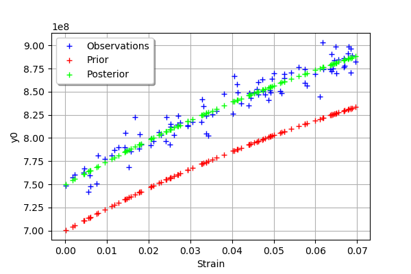
graph = mypcr.drawObservationsVsInputs()
graph.setLegendPosition("topleft")
graph

[20]:

../../_images/examples_calibration_calibration_chaboche_39_0.png

We see that there is a good fit after calibration, since the predictions after calibration (i.e. the green crosses) are close to the observations (i.e. the blue crosses).

[21]:

mypcr.drawObservationsVsPredictions()

[21]:

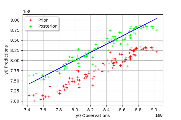
../../_images/examples_calibration_calibration_chaboche_41_0.png

We see that there is a much better fit after calibration, since the predictions are close to the diagonal of the graphics.

[22]:

observationError = calibrationResult.getObservationsError()
observationError

[22]:

Normal(mu = 0, sigma = 1.10416e+07)

[23]:

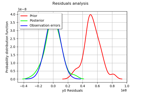
graph = mypcr.drawResiduals()
graph.setLegendPosition("topleft")
graph

[23]:

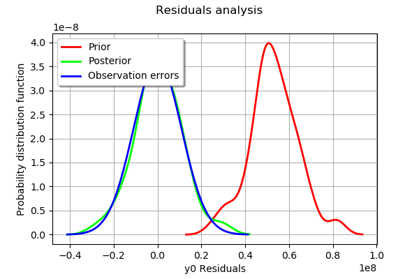
../../_images/examples_calibration_calibration_chaboche_44_0.png

The analysis of the residuals shows that the distribution is centered on zero and symmetric. This indicates that the calibration performed well.

Moreover, the distribution of the residuals is close to being gaussian.

[24]:

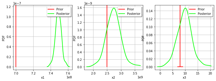
_ = mypcr.drawParameterDistributions()

../../_images/examples_calibration_calibration_chaboche_46_0.png

Calibration with nonlinear least squares¶

The NonLinearLeastSquaresCalibration class performs the non linear least squares calibration by minimizing the squared euclidian norm between the predictions and the observations.

[25]:

algo = ot.NonLinearLeastSquaresCalibration(mycf, observedStrain, observedStress, thetaPrior)

The run method computes the solution of the problem.

[26]:

algo.run()

[27]:

calibrationResult = algo.getResult()

Analysis of the results¶

The getParameterMAP method returns the maximum of the posterior distribution of $\theta$ .

[28]:

thetaMAP = calibrationResult.getParameterMAP()
thetaMAP

[28]:

[7.48444e+08,2.74804e+09,9.78149]

We can compute a 95% confidence interval of the parameter $\theta^\star$ .

[29]:

thetaPosterior = calibrationResult.getParameterPosterior()
thetaPosterior.computeBilateralConfidenceIntervalWithMarginalProbability(0.95)[0]

[29]:

[7.40173e+08, 7.57679e+08]
[2.11479e+09, 3.48123e+09]
[2.9595, 17.3487]

We can see that all three parameters are estimated with a large confidence interval.

[30]:

mypcr = CalibrationAnalysis(calibrationResult,mycf, observedStrain, observedStress)

[31]:

graph = mypcr.drawObservationsVsInputs()
graph.setLegendPosition("topleft")
graph

[31]:

../../_images/examples_calibration_calibration_chaboche_60_0.png

We see that there is a good fit after calibration, since the predictions after calibration (i.e. the green crosses) are close to the observations (i.e. the blue crosses).

[32]:

mypcr.drawObservationsVsPredictions()

[32]:

../../_images/examples_calibration_calibration_chaboche_62_0.png

We see that there is a much better fit after calibration, since the predictions are close to the diagonal of the graphics.

[33]:

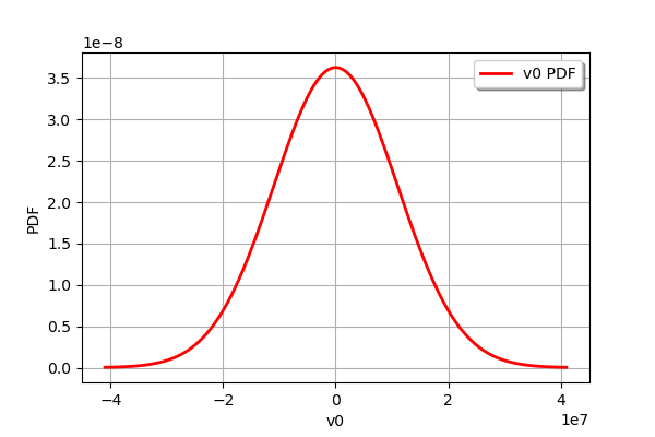
observationError = calibrationResult.getObservationsError()
observationError

[33]:

Normal(mu = 3573.98, sigma = 1.09955e+07)

[34]:

observationError.drawPDF()

[34]:

../../_images/examples_calibration_calibration_chaboche_65_0.png

[35]:

graph = mypcr.drawResiduals()
graph.setLegendPosition("topleft")
graph

[35]:

../../_images/examples_calibration_calibration_chaboche_66_0.png

The analysis of the residuals shows that the distribution is centered on zero and symmetric. This indicates that the calibration performed well.

Moreover, the distribution of the residuals is close to being gaussian. This indicates that the observation error might be gaussian.

[36]:

_ = mypcr.drawParameterDistributions()

../../_images/examples_calibration_calibration_chaboche_68_0.png

Gaussian calibration parameters¶

The standard deviation of the observations errors.

[37]:

sigmaStress = 1.e7 # (Pa)

Define the covariance matrix of the output Y of the model.

[38]:

errorCovariance = ot.CovarianceMatrix(1)
errorCovariance[0,0] = sigmaStress**2

Define the covariance matrix of the parameters $\theta$ to calibrate.

[39]:

sigmaR = 0.1 * R
sigmaC = 0.1 * C
sigmaGamma = 0.1 * Gamma

[40]:

sigma = ot.CovarianceMatrix(3)
sigma[0,0] = sigmaR**2
sigma[1,1] = sigmaC**2
sigma[2,2] = sigmaGamma**2
sigma

[40]:

[[ 4.9e+15 0 0 ]
[ 0 6.25e+16 0 ]
[ 0 0 0.64 ]]

Gaussian linear calibration¶

The GaussianLinearCalibration class performs the gaussian linear calibration by linearizing the model in the neighbourhood of the prior.

[41]:

algo = ot.GaussianLinearCalibration(mycf, observedStrain, observedStress, thetaPrior, sigma, errorCovariance)

The run method computes the solution of the problem.

[42]:

algo.run()

[43]:

calibrationResult = algo.getResult()

Analysis of the results¶

The getParameterMAP method returns the maximum of the posterior distribution of $\theta$ .

[44]:

thetaMAP = calibrationResult.getParameterMAP()
thetaMAP

[44]:

[7.49845e+08,2.60366e+09,8.15841]

We can compute a 95% confidence interval of the parameter $\theta^\star$ .

[45]:

thetaPosterior = calibrationResult.getParameterPosterior()
thetaPosterior.computeBilateralConfidenceIntervalWithMarginalProbability(0.95)[0]

[45]:

[7.44583e+08, 7.55108e+08]
[2.40769e+09, 2.79962e+09]
[6.45772, 9.8591]

We can see that all three parameters are estimated with a large confidence interval.

[46]:

mypcr = CalibrationAnalysis(calibrationResult,mycf,observedStrain, observedStress)

[47]:

graph = mypcr.drawObservationsVsInputs()
graph.setLegendPosition("topleft")
graph

[47]:

../../_images/examples_calibration_calibration_chaboche_90_0.png

We see that there is a good fit after calibration, since the predictions after calibration (i.e. the green crosses) are close to the observations (i.e. the blue crosses).

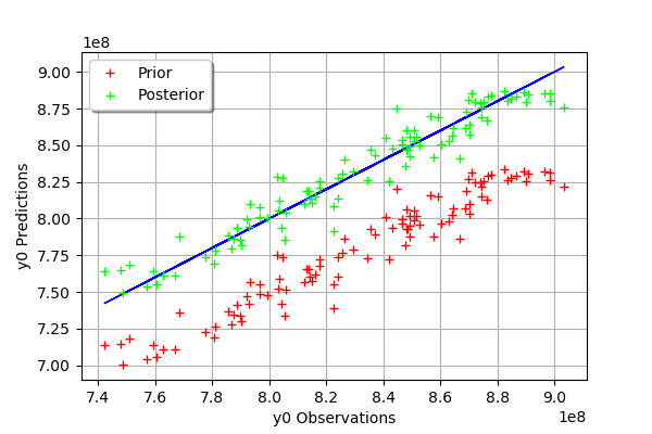
[48]:

mypcr.drawObservationsVsPredictions()

[48]:

../../_images/examples_calibration_calibration_chaboche_92_0.png

We see that there is a much better fit after calibration, since the predictions are close to the diagonal of the graphics.

The observation error is predicted by linearizing the problem at the prior.

[49]:

observationError = calibrationResult.getObservationsError()
observationError

[49]:

Normal(mu = 0, sigma = 1e+07)

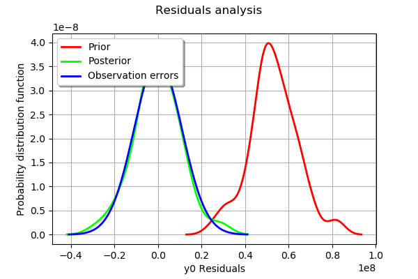
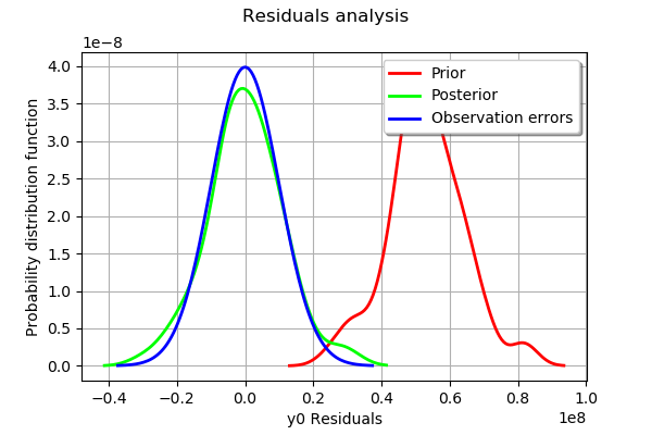
This can be compared to the residuals distribution, which is computed at the posterior.

[50]:

graph = mypcr.drawResiduals()
graph.setLegendPosition("topleft")
graph

[50]:

../../_images/examples_calibration_calibration_chaboche_97_0.png

The analysis of the gaussian distribution (the blue line) of the observation errors is close to the posterior distribution of the residuals (the green line). Moreover, the posterior distribution is centered. These informations indicate that the calibration performed well.

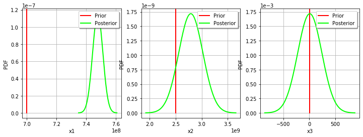
[51]:

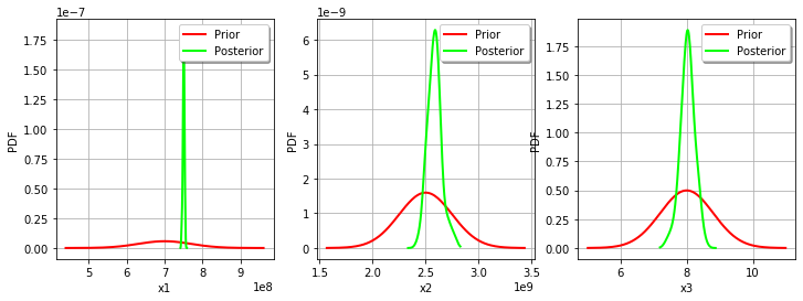
_ = mypcr.drawParameterDistributions()

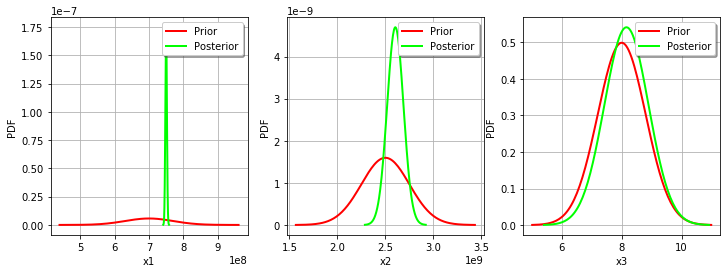
../../_images/examples_calibration_calibration_chaboche_99_0.png

For the $R$ variable, the observations are much more important than the prior: this is shown by the fact that the posterior and prior distribution of the $R$ variable are very different.

We see that the prior and posterior distribution are close to each other for the $\gamma$ variable: the observations did not convey much information for this variable.

Gaussian nonlinear calibration¶

The GaussianNonLinearCalibration class performs the gaussian nonlinear calibration.

[52]:

algo = ot.GaussianNonLinearCalibration(mycf, observedStrain, observedStress, thetaPrior, sigma, errorCovariance)

The run method computes the solution of the problem.

[53]:

algo.run()

[54]:

calibrationResult = algo.getResult()

Analysis of the results¶

The getParameterMAP method returns the maximum of the posterior distribution of $\theta$ .

[55]:

thetaMAP = calibrationResult.getParameterMAP()
thetaMAP

[55]:

[7.50434e+08,2.58012e+09,8.02108]

We can compute a 95% confidence interval of the parameter $\theta^\star$ .

[56]:

thetaPosterior = calibrationResult.getParameterPosterior()
thetaPosterior.computeBilateralConfidenceIntervalWithMarginalProbability(0.95)[0]

[56]:

[7.44106e+08, 7.55416e+08]
[2.42955e+09, 2.77875e+09]
[7.41359, 8.55092]

We can see that all three parameters are estimated with a large confidence interval.

[57]:

mypcr = CalibrationAnalysis(calibrationResult,mycf, observedStrain, observedStress)

[58]:

graph = mypcr.drawObservationsVsInputs()
graph.setLegendPosition("topleft")
graph

[58]:

../../_images/examples_calibration_calibration_chaboche_114_0.png

We see that there is a good fit after calibration, since the predictions after calibration (i.e. the green crosses) are close to the observations (i.e. the blue crosses).

[59]:

mypcr.drawObservationsVsPredictions()

[59]:

../../_images/examples_calibration_calibration_chaboche_116_0.png

We see that there is a much better fit after calibration, since the predictions are close to the diagonal of the graphics.

The observation error is predicted by bootstraping the problem at the posterior.

[60]:

observationError = calibrationResult.getObservationsError()
observationError

[60]:

Normal(mu = 0, sigma = 1e+07)

This can be compared to the residuals distribution, which is computed at the posterior.

[61]:

mypcr.drawResiduals()

[61]:

../../_images/examples_calibration_calibration_chaboche_121_0.png

The analysis is very similar to the linear calibration.

[62]:

_ = mypcr.drawParameterDistributions()

../../_images/examples_calibration_calibration_chaboche_123_0.png

We see that the prior and posterior distribution for the $\gamma$ parameter are close to each other, but not superimposed: the observations significantly brought information to the variable $\gamma$ during the calibration.

OpenTURNS

An Open source initiative for the Treatment of Uncertainties, Risks'N Statistics

Table of Contents

Previous topic

Next topic

This Page

Calibration of the Chaboche mecanical model¶

Deterministic model¶

Parameters to calibrate¶

Observations¶

Thanks to¶

References¶

Generate the observations¶

A calibration analysis class¶

Set the calibration parameters¶

Calibration with linear least squares¶

Analysis of the results¶

Calibration with nonlinear least squares¶

Analysis of the results¶

Gaussian calibration parameters¶

Gaussian linear calibration¶

Analysis of the results¶

Gaussian nonlinear calibration¶

Analysis of the results¶