Compare unconditional and conditional histograms¶

In this example, we compare unconditional and conditional histograms for a simulation. We consider the flooding model. Let $g$ be a function which takes four inputs $Q$ , $K_s$ , $Z_v$ and $Z_m$ and returns one output $H$ .

We first consider the (unconditional) distribution of the input $Q$ .

Let $t$ be a given threshold on the output $H$ : we consider the event $H>t$ . Then we consider the conditional distribution of the input $Q$ given that $H>t$ : $Q|H>t$ .

If these two distributions are significantly different, we conclude that the input $Q$ has an impact on the event $H>t$ .

In order to approximate the distribution of the output $H$ , we perform a Monte-Carlo simulation with size 500. The threshold $t$ is chosen as the 90% quantile of the empirical distribution of $H$ . In this example, the distribution is aproximated by its empirical histogram (but this could be done with another distribution approximation as well, such as kernel smoothing for example).

[1]:

import openturns as ot

Create the marginal distributions of the parameters.

[2]:

dist_Q = ot.TruncatedDistribution(ot.Gumbel(558., 1013.), 0, ot.TruncatedDistribution.LOWER)
dist_Ks = ot.TruncatedDistribution(ot.Normal(30.0, 7.5), 0, ot.TruncatedDistribution.LOWER)
dist_Zv = ot.Uniform(49.0, 51.0)
dist_Zm = ot.Uniform(54.0, 56.0)
marginals = [dist_Q, dist_Ks, dist_Zv, dist_Zm]

Create the joint probability distribution.

[3]:

distribution = ot.ComposedDistribution(marginals)
distribution.setDescription(['Q', 'Ks', 'Zv', 'Zm'])

Create the model.

[4]:

model = ot.SymbolicFunction(['Q', 'Ks', 'Zv', 'Zm'],
                            ['(Q/(Ks*300.*sqrt((Zm-Zv)/5000)))^(3.0/5.0)'])

Create a sample.

[5]:

size = 500
inputSample = distribution.getSample(size)
outputSample = model(inputSample)

Merge the input and output samples into a single sample.

[6]:

sample = ot.Sample(size,5)
sample[:,0:4] = inputSample
sample[:,4] = outputSample
sample[0:5,:]

[6]:

	v0	v1	v2	v3	v4
0	1443.602798325532	30.156613494725274	49.11713595070338	55.59185930777356	2.4439424253360924
1	2174.8898945480146	34.67890291392808	50.764851072298455	55.87647205461956	3.085132426791521
2	626.1023680891167	35.75352992912951	50.03020209989136	54.661879004882564	1.478061905093236
3	325.8123641551359	36.665987740324184	49.026338291130784	55.366752716918725	0.8953760185932061
4	981.3994326290226	41.10229410031924	49.39776320365176	54.84770660838047	1.6954636957219766

Extract the first column of inputSample into the sample of the flowrates $Q$ .

[7]:

sampleQ = inputSample[:,0]

[8]:

import numpy as np

def computeConditionnedSample(sample, alpha = 0.9, criteriaComponent = None, selectedComponent = 0):
    '''
    Return values from the selectedComponent-th component of the sample.
    Selects the values according to the alpha-level quantile of
    the criteriaComponent-th component of the sample.
    '''
    dim = sample.getDimension()
    if criteriaComponent is None:
        criteriaComponent = dim - 1
    sortedSample = sample.sortAccordingToAComponent(criteriaComponent)
    quantiles = sortedSample.computeQuantilePerComponent(alpha)
    quantileValue = quantiles[criteriaComponent]
    sortedSampleCriteria = sortedSample[:,criteriaComponent]
    indices = np.where(np.array(sortedSampleCriteria.asPoint())>quantileValue)[0]
    conditionnedSortedSample = sortedSample[int(indices[0]):,selectedComponent]
    return conditionnedSortedSample

Create an histogram for the unconditional flowrates.

[9]:

numberOfBins = 10
histogram = ot.HistogramFactory().buildAsHistogram(sampleQ,numberOfBins)

Extract the sub-sample of the input flowrates Q which leads to large values of the output H.

[10]:

alpha = 0.9
criteriaComponent = 4
selectedComponent = 0
conditionnedSampleQ = computeConditionnedSample(sample,alpha,criteriaComponent,selectedComponent)

We could as well use:

conditionnedHistogram = ot.HistogramFactory().buildAsHistogram(conditionnedSampleQ)

but this creates an histogram with new classes, corresponding to conditionnedSampleQ. We want to use exactly the same classes as the full sample, so that the two histograms match.

[11]:

first = histogram.getFirst()
width = histogram.getWidth()
conditionnedHistogram = ot.HistogramFactory().buildAsHistogram(conditionnedSampleQ,first,width)

Then creates a graphics with the unconditional and the conditional histograms.

[12]:

graph = histogram.drawPDF()
graph.setLegends(["Q"])
#
graphConditionnalQ = conditionnedHistogram.drawPDF()
graphConditionnalQ.setColors(["blue"])
graphConditionnalQ.setLegends(["Q|H>H_%s" % (alpha)])
graph.add(graphConditionnalQ)
graph

[12]:

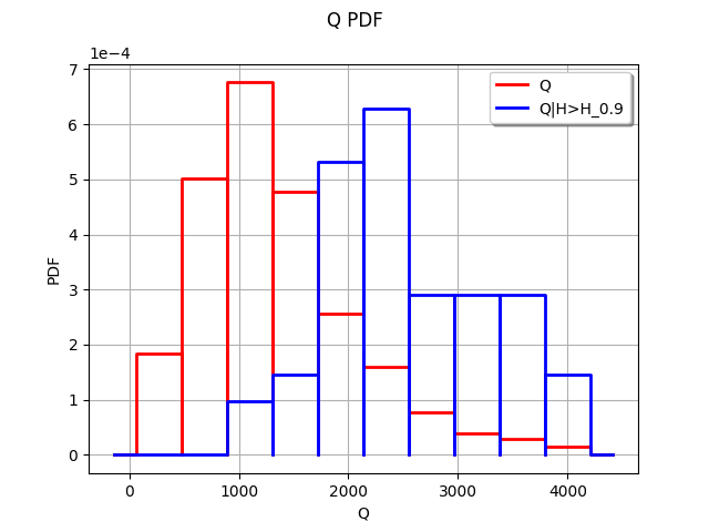
../../_images/examples_data_analysis_compare_unconditional_conditional_histograms_23_0.png

We see that the two histograms are very different. The high values of the input $Q$ seem to often lead to a high value of the output $H$ .

We could explore this situation further by comparing the unconditional distribution of $Q$ (which is known in this case) with the conditonal distribution of $Q|H>t$ , estimated by kernel smoothing. This would have the advantage of accuracy, since the kernel smoothing is a more accurate approximation of a distribution than the histogram.

OpenTURNS

An Open source initiative for the Treatment of Uncertainties, Risks'N Statistics

Previous topic

Next topic

This Page

Compare unconditional and conditional histograms¶