Define a function with a field output: the viscous free fall example
In this example, we define a function which has a vector input and a field output. This is why we use the PythonPointToFieldFunction class to create the associated function and propagate the uncertainties through it.
Introduction
We consider an object inside a vertical cylinder which contains a viscous fluid. The fluid generates a drag force which limits the speed of the solid and we assume that the force depends linearily on the object speed:

for any ![t \in [0, t_{max}]](../../_images/math/e37ccc57d86c6e709093d85dc5d9560d5abd78e3.svg) where:
where:
 is the speed
 ![[m/s]](../../_images/math/3e089dba72d0221acb9cd7e65dec1e8f109be9c5.svg) ,
, is the time
 ![[s]](../../_images/math/e4ad022bfc97738d014806873e944cabafc5e09e.svg) ,
, is the maximum time ,
 is the gravitational acceleration
 ![[m.s^{-2}]](../../_images/math/8a142fffbe98732eea43f29b9337046e11be81e6.svg) ,
, is the mass
 ![[kg]](../../_images/math/4de6be7753609caccb2680c56747b51534b6d4b0.svg) ,
, is the linear drag coefficient
 ![[kg.s^{-1}]](../../_images/math/57b592d441c8146a60c6eea6e61b7c3e693988ab.svg) .
.
The previous differential equation has the exact solution:

for any
where:
 is the altitude above the surface
 ![[m]](../../_images/math/aa7e8a983b183cd5f9697f35d4902d7d6f55dc5a.svg) ,
, is the initial altitude ,
 is the initial speed (upward)
 ![[m.s^{-1}]](../../_images/math/5d3f566646a0a1c98c5b8602556a0bf0d1f617db.svg) ,
, is the limit speed :

 is time caracteristic :

The stationnary speed limit at infinite time is equal to :

When there is no drag, i.e. when  , the trajectory depends quadratically on :

for any .
Furthermore when the solid touches the ground, we ensure that the altitude remains nonnegative i.e. the final altitude is:

for any .
 ,
, ,
, ,
, .
.References
Steven C. Chapra. Applied numerical methods with Matlab for engineers and scientists, Third edition. 2012. Chapter 7, “Optimization”, p.182.
Define the model
[1]:
from __future__ import print_function
import openturns as ot
import numpy as np
We first define the time grid associated with the model.
[2]:
tmin=0.0 # Minimum time
tmax=12. # Maximum time
gridsize=100 # Number of time steps
mesh = ot.IntervalMesher([gridsize-1]).build(ot.Interval(tmin, tmax))
The getVertices method returns the time values in this mesh.
[3]:
vertices = mesh.getVertices()
vertices[0:5]
[3]:
| v0 | |
|---|---|
| 0 | 0.0 |
| 1 | 0.12121212121212122 |
| 2 | 0.24242424242424243 |
| 3 | 0.36363636363636365 |
| 4 | 0.48484848484848486 |
Creation of the input distribution.
[4]:
distZ0 = ot.Uniform(100.0, 150.0)
distV0 = ot.Normal(55.0, 10.0)
distM = ot.Normal(80.0, 8.0)
distC = ot.Uniform(0.0, 30.0)
distribution = ot.ComposedDistribution([distZ0, distV0, distM, distC])
[5]:
dimension = distribution.getDimension()
dimension
[5]:
4
Then we define the Python function which computes the altitude at each time value. In order to compute all altitudes with a vectorized evaluation, we first convert the vertices into a numpy array and use the numpy function exp and maximum: this increases the evaluation performance of the script.
[6]:
def AltiFunc(X):
    g  = 9.81
    z0 = X[0]
    v0 = X[1]
    m  = X[2]
    c  = X[3]
    tau = m / c
    vinf = - m * g / c
    t = np.array(vertices)
    z = z0 + vinf * t + tau * (v0 - vinf) * (1 - np.exp( - t / tau))
    z = np.maximum(z,0.)
    return [[zeta[0]] for zeta in z]
In order to create a Function from this Python function, we use the PythonPointToFieldFunction class. Since the altitude is the only output field, the third argument outputDimension is equal to 1. If we had computed the speed as an extra output field, we would have set 2 instead.
[7]:
outputDimension = 1
alti = ot.PythonPointToFieldFunction(dimension, mesh, outputDimension, AltiFunc)
Sample trajectories
In order to sample trajectories, we use the getSample method of the input distribution and apply the field function.
[8]:
size = 10
inputSample = distribution.getSample(size)
outputSample = alti(inputSample)
[9]:
ot.ResourceMap.SetAsUnsignedInteger('Drawable-DefaultPalettePhase', size)
Draw some curves.
[10]:
graph = outputSample.drawMarginal(0)
graph.setTitle('Viscous free fall: %d trajectories' % (size))
graph.setXTitle(r'$t$')
graph.setYTitle(r'$z$')
graph
[10]:
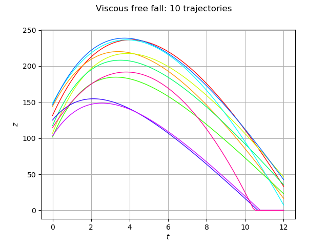
We see that the object first moves up and then falls down. Not all objects, however, achieve the same maximum altitude. We see that some trajectories reach a higher maximum altitude than others. Moreover, at the final time , one trajectory hits the ground:  for this trajectory.