Compare unconditional and conditional histograms

In this example, we compare unconditional and conditional histograms for a simulation. We consider the flooding model. Let be a function which takes four inputs , , and and returns one output .

We first consider the (unconditional) distribution of the input .

Let be a given threshold on the output : we consider the event . Then we consider the conditional distribution of the input given that : .

If these two distributions are significantly different, we conclude that the input has an impact on the event .

In order to approximate the distribution of the output , we perform a Monte-Carlo simulation with size 500. The threshold is chosen as the 90% quantile of the empirical distribution of . In this example, the distribution is aproximated by its empirical histogram (but this could be done with another distribution approximation as well, such as kernel smoothing for example).

import openturns as ot
import openturns.viewer as viewer
from matplotlib import pylab as plt
ot.Log.Show(ot.Log.NONE)

We use the FloodModel data class that contains all the case parameters.

from openturns.usecases import flood_model as flood_model
fm = flood_model.FloodModel()

Create an input sample from the joint distribution defined in the data class. We build an output sample by taking the image by the model.

size = 500
inputSample = fm.distribution.getSample(size)
outputSample = fm.model(inputSample)

Merge the input and output samples into a single sample.

sample = ot.Sample(size,5)
sample[:,0:4] = inputSample
sample[:,4] = outputSample
sample[0:5,:]

	v0	v1	v2	v3	v4
0	2032.978	28.16431	49.81823	54.44882	-5.224069
1	831.1784	32.06598	49.8578	54.29531	-6.747824
2	1741.776	19.36681	49.08975	55.0745	-5.757122
3	800.476	40.00743	49.16216	55.03673	-7.846938
4	917.9835	38.23018	49.19878	54.97124	-7.629101

Extract the first column of inputSample into the sample of the flowrates .

sampleQ = inputSample[:,0]

import numpy as np

def computeConditionnedSample(sample, alpha = 0.9, criteriaComponent = None, selectedComponent = 0):
    '''
    Return values from the selectedComponent-th component of the sample.
    Selects the values according to the alpha-level quantile of
    the criteriaComponent-th component of the sample.
    '''
    dim = sample.getDimension()
    if criteriaComponent is None:
        criteriaComponent = dim - 1
    sortedSample = sample.sortAccordingToAComponent(criteriaComponent)
    quantiles = sortedSample.computeQuantilePerComponent(alpha)
    quantileValue = quantiles[criteriaComponent]
    sortedSampleCriteria = sortedSample[:,criteriaComponent]
    indices = np.where(np.array(sortedSampleCriteria.asPoint())>quantileValue)[0]
    conditionnedSortedSample = sortedSample[int(indices[0]):,selectedComponent]
    return conditionnedSortedSample

Create an histogram for the unconditional flowrates.

numberOfBins = 10
histogram = ot.HistogramFactory().buildAsHistogram(sampleQ,numberOfBins)

Extract the sub-sample of the input flowrates Q which leads to large values of the output H.

alpha = 0.9
criteriaComponent = 4
selectedComponent = 0
conditionnedSampleQ = computeConditionnedSample(sample,alpha,criteriaComponent,selectedComponent)

We could as well use: ` conditionnedHistogram = ot.HistogramFactory().buildAsHistogram(conditionnedSampleQ) ` but this creates an histogram with new classes, corresponding to conditionnedSampleQ. We want to use exactly the same classes as the full sample, so that the two histograms match.

first = histogram.getFirst()
width = histogram.getWidth()
conditionnedHistogram = ot.HistogramFactory().buildAsHistogram(conditionnedSampleQ,first,width)

Then creates a graphics with the unconditional and the conditional histograms.

graph = histogram.drawPDF()
graph.setLegends(["Q"])
#
graphConditionnalQ = conditionnedHistogram.drawPDF()
graphConditionnalQ.setColors(["blue"])
graphConditionnalQ.setLegends([r"$Q|H>H_{%s}$" % (alpha)])
graph.add(graphConditionnalQ)
view = viewer.View(graph)

plt.show()

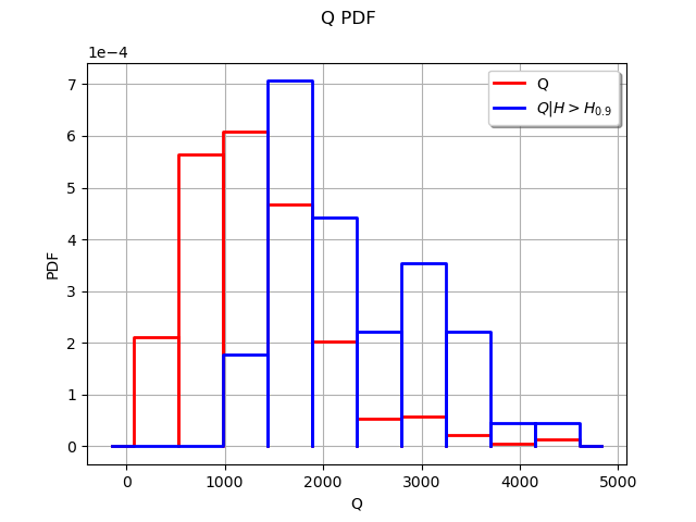
We see that the two histograms are very different. The high values of the input seem to often lead to a high value of the output .

We could explore this situation further by comparing the unconditional distribution of (which is known in this case) with the conditonal distribution of , estimated by kernel smoothing. This would have the advantage of accuracy, since the kernel smoothing is a more accurate approximation of a distribution than the histogram.