Define a function with a field output: the viscous free fall example

In this example, we define a function which has a vector input and a field output. This is why we use the PythonPointToFieldFunction class to create the associated function and propagate the uncertainties through it.

We consider a viscous free fall as explained here.

Define the model

from __future__ import print_function
import openturns as ot
import openturns.viewer as viewer
from matplotlib import pylab as plt
import numpy as np
ot.Log.Show(ot.Log.NONE)

We first define the time grid associated with the model.

tmin=0.0 # Minimum time
tmax=12. # Maximum time
gridsize=100 # Number of time steps
mesh = ot.IntervalMesher([gridsize-1]).build(ot.Interval(tmin, tmax))

The getVertices method returns the time values in this mesh.

vertices = mesh.getVertices()
vertices[0:5]

	v0
0	0
1	0.1212121
2	0.2424242
3	0.3636364
4	0.4848485

Creation of the input distribution.

distZ0 = ot.Uniform(100.0, 150.0)
distV0 = ot.Normal(55.0, 10.0)
distM = ot.Normal(80.0, 8.0)
distC = ot.Uniform(0.0, 30.0)
distribution = ot.ComposedDistribution([distZ0, distV0, distM, distC])

dimension = distribution.getDimension()
dimension

Out:

4

Then we define the Python function which computes the altitude at each time value. In order to compute all altitudes with a vectorized evaluation, we first convert the vertices into a numpy array and use the numpy function exp and maximum: this increases the evaluation performance of the script.

def AltiFunc(X):
    g  = 9.81
    z0 = X[0]
    v0 = X[1]
    m  = X[2]
    c  = X[3]
    tau = m / c
    vinf = - m * g / c
    t = np.array(vertices)
    z = z0 + vinf * t + tau * (v0 - vinf) * (1 - np.exp( - t / tau))
    z = np.maximum(z,0.)
    return [[zeta[0]] for zeta in z]

In order to create a Function from this Python function, we use the PythonPointToFieldFunction class. Since the altitude is the only output field, the third argument outputDimension is equal to 1. If we had computed the speed as an extra output field, we would have set 2 instead.

outputDimension = 1
alti = ot.PythonPointToFieldFunction(dimension, mesh, outputDimension, AltiFunc)

Sample trajectories

In order to sample trajectories, we use the getSample method of the input distribution and apply the field function.

size = 10
inputSample = distribution.getSample(size)
outputSample = alti(inputSample)

ot.ResourceMap.SetAsUnsignedInteger('Drawable-DefaultPalettePhase', size)

Draw some curves.

graph = outputSample.drawMarginal(0)
graph.setTitle('Viscous free fall: %d trajectories' % (size))
graph.setXTitle(r'$t$')
graph.setYTitle(r'$z$')
view = viewer.View(graph)
plt.show()

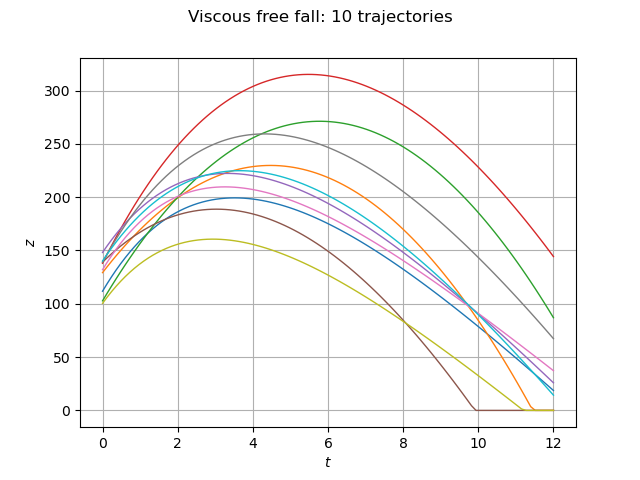
We see that the object first moves up and then falls down. Not all objects, however, achieve the same maximum altitude. We see that some trajectories reach a higher maximum altitude than others. Moreover, at the final time , one trajectory hits the ground: for this trajectory.